#首先导入ape
if(!require(ape)){
    install.packages("ape")  #'ape' will be installed if needed
    library(ape)
}
tree使用 “phylo” 类
我们使用 rtree() function 生成一个树,参数 n= 30个 tips (可以理解为末端节点)
phy <- rtree(n=30)    #n specifies the number of tips we want.
plot(phy)
查看树是由哪些数据构成的,我们先来理解下“phylo”类
class(phy)     #查看phy类型
## [1] "phylo"

phy   #包含30个tips 和29个内部节点(可以理解为树的分叉点)
## Phylogenetic tree with 30 tips and 29 internal nodes.
##
## Tip labels:
##  t13, t28, t8, t22, t19, t16, ...
##
## Rooted; includes branch lengths.
str(phy)  #其实phy类似于list类型
## List of 4
##  $ edge       : int [1:58, 1:2] 31 32 33 34 35 36 37 37 38 38 ...
##  $ tip.label  : chr [1:30] "t13" "t28" "t8" "t22" ...
##  $ edge.length: num [1:58] 0.2235 0.4492 0.0535 0.9588 0.2777 ...
##  $ Nnode      : int 29
##  - attr(*, "class")= chr "phylo"
##  - attr(*, "order")= chr "cladewise"
依次来看一下各数据结构及代表什么
head(phy$edge)    #一个两列的数据框
##      [,1] [,2]
## [1,]   31   32
## [2,]   32   33
## [3,]   33   34
##  ..

phy$tip.label    #树末端的label
##  [1] "t13" "t28" "t8"  "t22" "t19" "t16" "t7"  "t11" "t4"  "t24" "t17"
## [12] "t26" "t15" "t1"  "t12" "t30" "t27" "t6"  "t29" "t3"  "t20" "t25"
## [23] "t10" "t21" "t23" "t14" "t18" "t9"  "t5"  "t2"

phy$edge.length   #树枝的长度
##  [1] 0.223515275 0.449214761 0.053517260 0.958796252 0.277726818
## ..
## [46] 0.339903616 0.173343718 0.993939807 0.176320243 0.087404924
## [51] 0.113624431 0.108095456 0.150655877 0.317285047 0.572281965
## [56] 0.019839419 0.529848145 0.998013315

phy$Nnode  #中间节点的个数
## [1] 29
Newick格式的tree文件
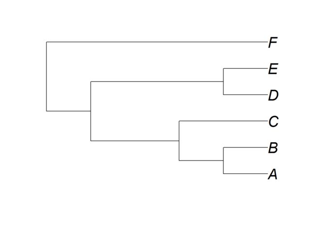
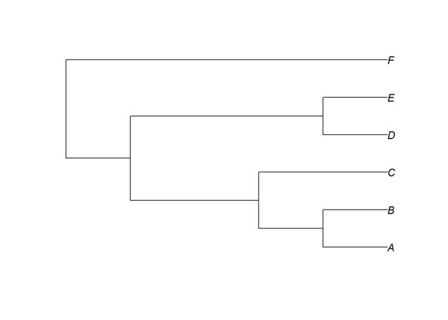
我们构建一个tips为 A-F的树,使用 read.tree()读取
mini.phy <- read.tree(text = "((((A,B), C), (D,E)),F);") #defining a tree in bracket form
plot(mini.phy, cex=2)
这个tree只包含3个数据,因为我们没提供edge的长度
str(mini.phy)
## List of 3
##  $ edge     : int [1:10, 1:2] 7 8 9 10 10 9 8 11 11 7 ...
##  $ tip.label: chr [1:6] "A" "B" "C" "D" ...
##  $ Nnode    : int 5
##  - attr(*, "class")= chr "phylo"
##  - attr(*, "order")= chr "cladewise"
我们看看这些边(edges)是怎么表示的
mini.phy$edge
##       [,1] [,2]
##  [1,]    7    8
##  [2,]    8    9
##  [3,]    9   10
##  [4,]   10    1
##  [5,]   10    2
##  [6,]    9    3
##  [7,]    8   11
##  [8,]   11    4
##  [9,]   11    5
## [10,]    7    6
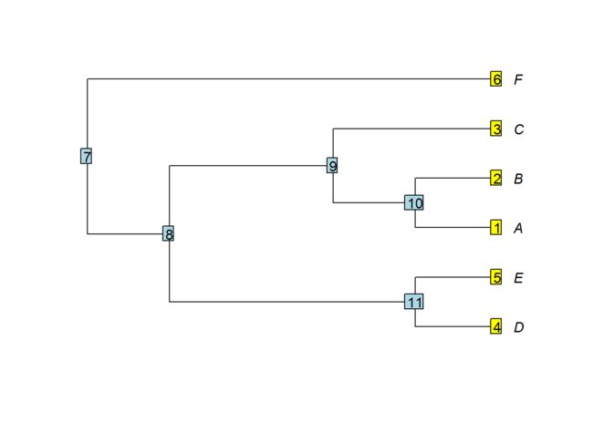
我们看到一个矩阵有10行和2列。这个矩阵表示节点和下一节点组合,定义了树的每一个分支。下面图中标出每个节点的数字
plot(mini.phy, label.offset=0.2)
nodelabels() #add node numbers
tiplabels()    #add tip numbers
使用tiplabels()给tip加上不同的颜色
mycol<-c("blue", "blue", "blue", "red", "red", "red") #颜色向量
plot(mini.phy, adj=0, label.offset=0.75)  #adjust if necessary/desired!
tiplabels(pch=21, col="black", adj=1, bg=mycol, cex=2) #ditto! try different values!
交换树枝的位置
有时旋转节点是很有必要的,使用rotate()function。继续使用mini.phy数据
plot(mini.phy, label.offset=0.2)   #same as before
nodelabels()  #add node numbers
tiplabels()   #add tip numbers
交换分支clades (D, E) and (A, B, C)? 图中可以看出他们的最近共同祖先是node 8.
rot.phy <- rotate(mini.phy, node=8)
plot(rot.phy, label.offset=0.2)   #still the same as before
nodelabels()
tiplabels()
找到指定分支下的所有tips,可以使用geiger包 的the tips() function得到分支下所有端点
library(geiger)
cladeABC <- tips(rot.phy, node=9) # node 9 defines the clade composed of (A, B, C)
cladeABC
## [1] "A" "B" "C"
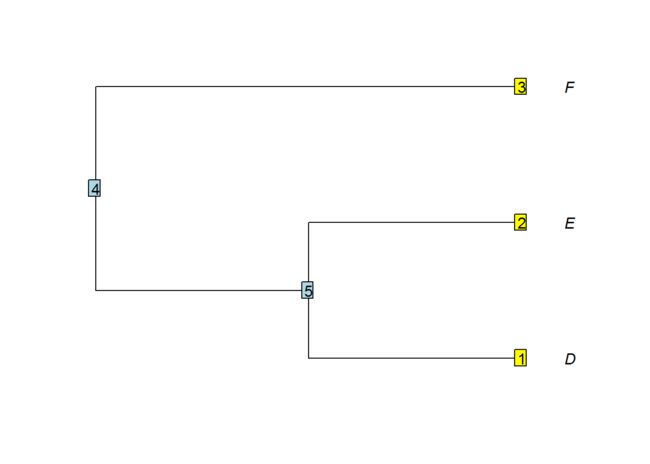
另外还有个修剪枝的函数drop.tip(),下面是剪切掉cladeABC分支
pruned.phy <- drop.tip(rot.phy, cladeABC)
plot(pruned.phy, label.offset=0.2)
nodelabels()
tiplabels() #did it work?
It may also be useful to select all branches in a specific group of tips. This is implemented in theapepackage; the which.edge() function finds all edges in a specified group. For example, let’s identify all branches of the cladeABC group as defined above.
cladeABCbranches <- which.edge(rot.phy, cladeABC)
#cladeABC was defined earlier, using the tips() function
cladeABCbranches #this should be a numerical vector containing 6, 7, 8, 9
## [1] 6 7 8 9
And as we can see, rows 6-9 of the
edge.length matrix represent the expected branches. Let’s first plot the tree, and then look at the edge matrix for cross-checking.
plot(rot.phy, label.offset=0.2) #we are sticking to the same plot settings
nodelabels()
tiplabels()
rot.phy$edge
##       [,1] [,2]
##  [1,]    7    8
##  [2,]    8   11
##  [3,]   11    4
##  [4,]   11    5
##  [5,]    8    9
##  [6,]    9   10
##  [7,]   10    1
##  [8,]   10    2
##  [9,]    9    3
## [10,]    7    6
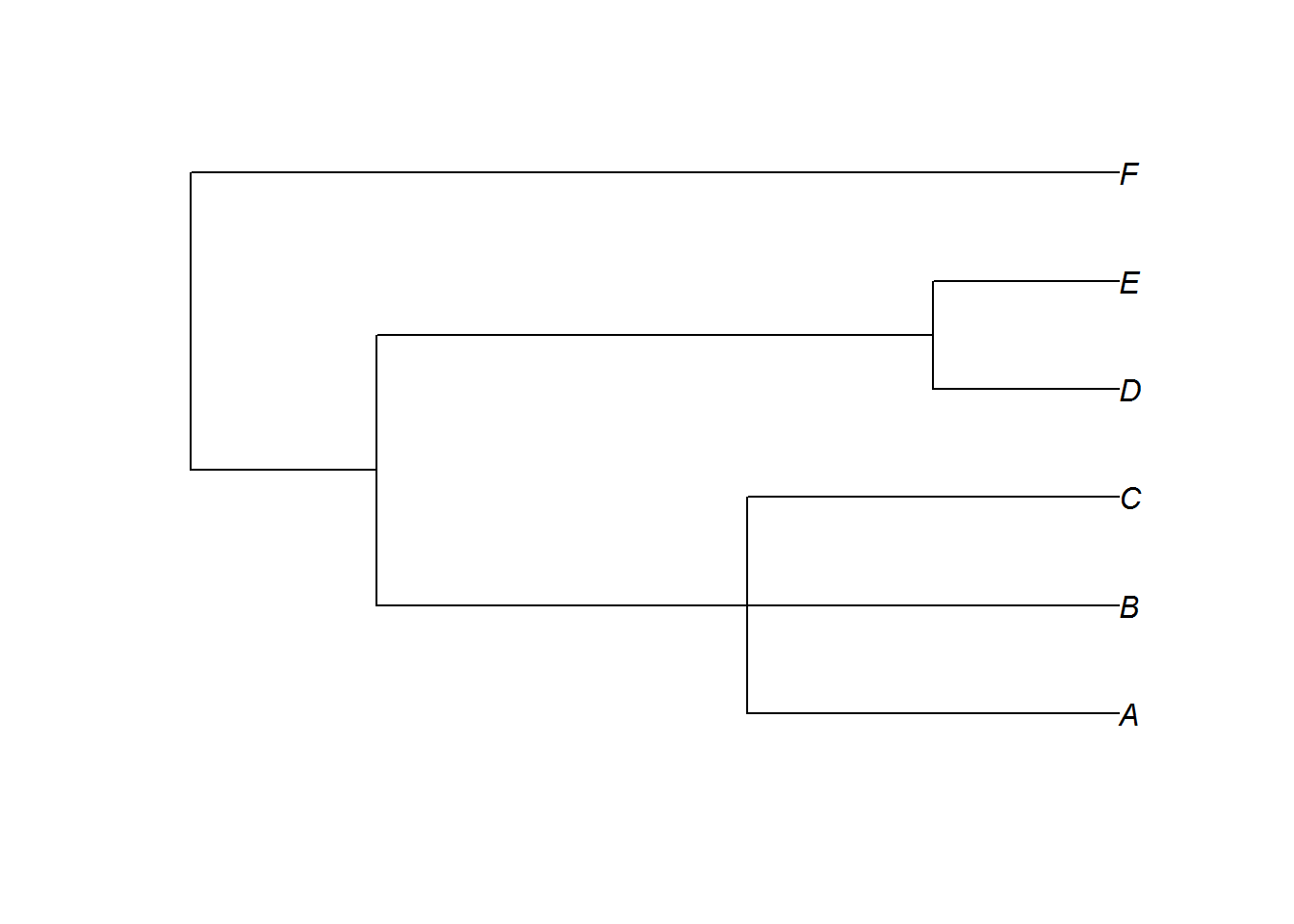
Here would be a good opportunity to show you how to assign different branch colors. For example, how can one emphasize the branches of the clade formed by A, B, and C? We first create a color vector, only consisting of grey colors. Then we’ll assign black to all branches of clade ABC.
clcolr <- rep("darkgrey", dim(rot.phy$edge)[1]) #defining a color vector; look up rep() and dim() functions!
clcolr[cladeABCbranches] <- "red" #specifying color of branches in clade (A, B, C)
lot(rot.phy, edge.color=clcolr, edge.width=2) #also making the branches a little thicker
Let’s conclude this section with one last exercise: combining trees. Assume you have two different phylogenies, with two different sets of taxa (no overlap). Another assumption is that you have knowledge how the trees may fit together. Then the bind.tree() function of ape package can help. The function takes in two phylo objects. The position of where the trees are bound is defined by tip- or node number within the first tree. Note that you can also specify the “root” as binding position.
#the first tree
tree1 <- rtree(n=10)
tree1$tip.label <- rep("apples", 10) #renaming labels to enhance readability
plot(tree1, label.offset=0.1); nodelabels(); tiplabels()
#the second tree
tree2 <- rtree(n=10)
tree2$tip.label <- rep("oranges", 10)
plot(tree2)
#merging trees
combined.tree <- bind.tree(tree1, tree2, where=5) #combining trees at position "5"
plot(combined.tree)
Try at least two different merging positions. For each example, plot the two original trees and the merged version in one figure.
Fully resolved and polytomous trees
All tree examples so far were fully resolved, i.e. each tree was fully binary. It’s very easy to access visually for small trees, but one can also do this more formally:
is.binary.tree(mini.phy)
## [1] TRUE
Let’s make a tree that is not fully resolved.
poly.phy <- read.tree(text = "(((A,B,C),(D,E)),F);") #A, B, and C form a polytomy
plot(poly.phy)
Is this tree binary?
is.binary.tree(poly.phy) # "FALSE"!
## [1] FALSE
OK. Many comparative methods require fully resolved trees. But what to do if that’s not the case? The multi2di() function can resolve polytomies, either randomly or in the order in which they appear in the tree. The default setting is to resolve polytomies randomly.
resolved.phy <- multi2di(poly.phy)
is.binary.tree(resolved.phy)
## [1] TRUE
plot(resolved.phy) # visual inspection.
If you repeat the above lines a few times you will see the effect of randomly resolving the polytomy.
Please plot two randomly resolved trees next to each other!
画图参数设置
通过修改参数,改变tree的样式
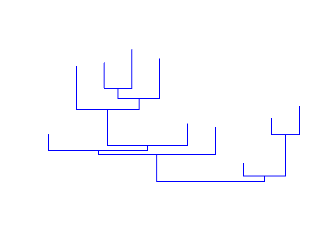
phy <- rtree(n=10) # n specifies the number of tips we want.
plot(phy) #default orientation is right-handed
plot(phy, direction="upwards",  # "rightwards" (default), "leftwards", and "downwards"
     show.tip.label=FALSE,  #显示tip.label
     #cex=.3       #tip.lable 字体大小
     edge.width=2,               #枝宽度
     edge.color="blue")       # 树枝颜色 ;蓝色
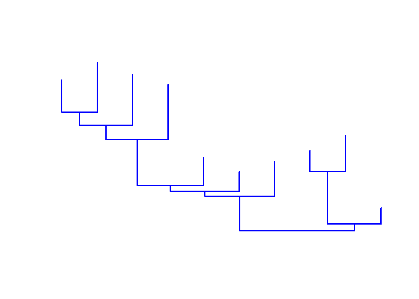
There are many other options… type ?plot.phylo in the console to read more. One last useful command I’d like to introduce is the ladderize() function. It reorganizes the tree structure, normally yielding much more readable trees.
ladderized.phy <- ladderize(phy)
plot(ladderized.phy, direction="upwards",
     show.tip.label=FALSE, edge.width=2, edge.color="blue")
来自:http://schmitzlab.info/phylo.html

