matlab中,在灰度解剖图上叠加阈值图,by by DR. Rajeev Raizada
1.参考 reference
1. tutorial主页:http://www.bcs.rochester.edu/people/raizada/fmri-matlab.htm。
2.speech_brain_images.mat数据:speech_brain_images.mat。
3.showing_brain_images_tutorial显示大脑图像代码:showing_brain_images_tutorial.m 。
4.overlaying_Tmaps_tutorial.m叠加t检验统计图:overlaying_Tmaps_tutorial.m。
2.程序执行过程 run step by step
目的:在灰度解剖图上叠加显示彩色阈值图。有一个难点:Unfortunately, it isn't quite that easy, because Matlab only lets you have one colormap per figure window.这里提出了这样的解决方案:就是把灰度图映射成真实的RGB真彩图。
2.1 对解剖图和功能图进行灰度值归一化,归一化至[1,64]区间,然后,将两个图像转成RGB图像,显示归一化后的解剖图,灰度方式显示,不是RGB:
%%%%%%% First, load in the file containing the brain images
load speech_brain_images.mat
%%%% Let's look at the 18th axial slice.
%%%% This goes through Heschl's gyrus, which is auditory cortex
axial_slice_number = 18;
%%%% Read the values from the 3D matrix subj_3danat
anat_slice_vals = subj_3danat(:,:,axial_slice_number);
%%%% Use squeeze to get rid of any redundant 3rd dimension that
%%%% might be left over. This is described in
%%%% more detail in showing_brain_images_tutorial.m
anat_slice_2D = squeeze(anat_slice_vals);
%%%% In order to make it easier for us to match up the
%%%% anatomical values to the 64-entries in Matlab's standard
%%%% gray colormap, we're going to scale the anatomical image
%%%% values so that they are all integers going from 1 to 64
%%%% First scale it from 0 to 1 by dividing by the maximum value.
%%%% Because it's a 2D matrix, we have to perform the max() operation
%%%% twice, once for each dimension. Then we end up with one max value,
%%%% which we can use as a divisor.
anat01 = anat_slice_2D ./ max(max(anat_slice_2D));
%%%% Next, multiply by 63 and round to the nearest whole number
anat0_63 = round( 63 * anat01 );
%%%% Finally, add 1, in order to make a matrix that goes from 1 to 64
anat64 = anat0_63 + 1;
%%%%%%%%%%%% Now let's do the same for the thresholded T-map
Tmap_slice_vals = speech_Tmap(:,:,axial_slice_number);
Tmap_slice_2D = squeeze(Tmap_slice_vals);
T_threshold = 1; %%% Let's pick a fairly low threshold, because it helps
%%% for showing the effect of transparent overlay later.
%%%% To threshold the map, make a logical 0/1 matrix that says
%%%% whether each voxel is above-threshold or not, and multiply
%%%% it element-by-element by the raw T-map values.
%%%% This is explained in a more step-by-step way
%%%% in the companion program showing_brain_images_tutorial.m
thresholded_Tmap = ( Tmap_slice_2D > T_threshold ) .* Tmap_slice_2D;
Tmap01 = thresholded_Tmap ./ max(max(thresholded_Tmap));
Tmap0_63 = round( 63 * Tmap01 );
Tmap64 = 1 + Tmap0_63;
%%%%%%%%%%%%%%%%%%%%%%%%%%%%%%%%%%%%%%%%%%%%%%%%%%%%%%%%%%%%%%%%
% Ok, now we have made two matrices scaled from 1 to 64,
% one for the anatomical image, and the other for the T-map image
%
% The next step is to make a full RGB-image for each image,
% by looking up the corresponding rows of the gray and hot colormaps.
%
% An RGB-image is a 3D-matrix.
% It has three "colour slabs" that are joined up along the third dimension.
% The first slab is an image full of Red values.
% The second slab is an image full of Green values.
% And the third slab is an image of Blue values.
% First make 3D matrices full of zeros, to hold the values
% that we are about to create for the anatomical and T-map RGB images.
% These have three slabs in the 3rd dimension, and are the same size as
% the anatomical and the Tmap matrices in the first two dimensions.
anat_RGB = zeros(size(anat64,1), size(anat64,2), 3);
%%% This will hold the anatomical image's RBG values
Tmap_RGB = zeros(size(Tmap64,1), size(Tmap64,2), 3);
%%% This will hold the T-map image's RBG values
%%% Now, let's get hold of copies of Matlab's gray and hot
%%% colormap matrices. As far as I know, we need to make a figure
%%% first in order to do this. That's fine, because we want to
%%% look at our newly created 1-to-64 scaled images anyway.
figure(1);
clf;
image(anat64); %%% Note that this is image(), not imagesc() !!!
%%% This looks the same as if we had used imagesc,
%%% because the image values are *already* scaled
%%% to cover the whole colormap, from black to white
colormap gray;
axis('image');
colorbar;
title('The anatomical image after we have scaled it from 1 to 64');
% Now that we are in colormap gray, let's make a copy of the colormap matrix
gray_cmap = colormap; %%% This reads in the current colormap matrix

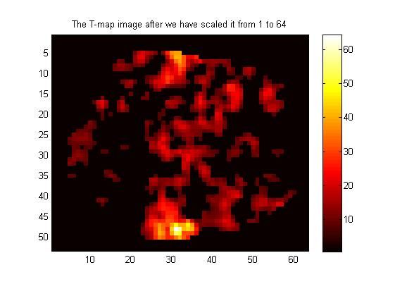
2.2 显示归一化后的功能图,hot方式显示,不是RGB:
figure(2);
clf;
image(Tmap64); %%% Again, note that we are using image(), not imagesc()
colormap hot;
axis('image');
colorbar;
title('The T-map image after we have scaled it from 1 to 64');
%%%%% Make a copy of the new current colormap matrix, which is now hot.
hot_cmap = colormap;
2.3 构造RGB解剖图,并按照RGB方式显示解剖图:
for RGB_dim = 1:3, %%% Loop through the three slabs: R, G, and B
%%% Each entry in each 1-to-64-scaled matrix gives us a row
%%% in the colormap matrix to go look-up.
%%% That row has three columns: the R, G and B values for that colour.
gray_cmap_rows_for_anat = anat64;
hot_cmap_rows_for_Tmap = Tmap64;
%%% We'll read in one of these R, G, or B values at a time,
%%% depending on which colour-slab we're building.
%%% The colormap entry we want is in the RGB_dim-th column,
%%% and in the row that we determined above.
%%% Note that we're actually looking up all the rows at once,
%%% because we're giving Matlab an entire matrix in the row-position.
colour_slab_vals_for_anat = gray_cmap(gray_cmap_rows_for_anat, RGB_dim);
colour_slab_vals_for_Tmap = hot_cmap(hot_cmap_rows_for_Tmap, RGB_dim);
%%%% These colour-slab values turn out to be in column vector format,
%%%% and need to be reshaped into being the same size as image matrices.
anat_RGB(:,:,RGB_dim) = reshape( colour_slab_vals_for_anat, size(anat64));
Tmap_RGB(:,:,RGB_dim) = reshape( colour_slab_vals_for_Tmap, size(Tmap64));
end; % End of loop through the RGB dimension.
%%%% Now that we've made our RGB images, let's look at them
%%%% Note that these types of images do *not* have colormaps.
%%%% Every image pixel has three numbers attached to it, not just one,
%%%% and those three numbers define the colour for that pixel directly,
%%%% by giving its R, G and B values.
figure(3);
clf;
image(anat_RGB);
axis('image');
title('The anatomical RGB image, with no colormap')

2.4 并按照RGB方式显示功能图:
figure(4);
clf;
image(Tmap_RGB);
axis('image');
title('The T-map RGB image, with no colormap')

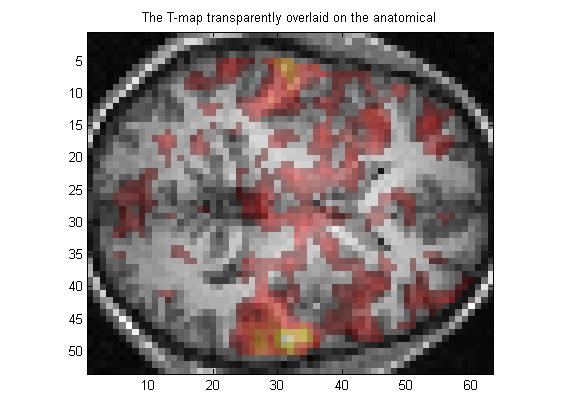
2.5 对阈值图做透明化处理,然后叠加到解剖图上:
Tmap_opacity = 0.4; % 0.4 is a reasonable opacity value to try first
%%%% Make a place-holder matrix to hold the compound weighted-sum image
compound_RGB = zeros(size(anat64,1), size(anat64,2), 3);
%%% The anat and the T-map are the same size,
%%% we could have chosen either.
%%% Now build up the compound image, one colour-slab at a time, like above.
%%% Where the T-map is below threshold, we only want the anatomical's values.
%%% Where the T-map is above-threshold, we want a weighted sum
%%% of the T-map RGB values and the anatomical's RGB values.
for RGB_dim = 1:3, %%% Loop through the three slabs: R, G, and B
compound_RGB(:,:,RGB_dim) = ...
(thresholded_Tmap==0) .* ... % Where T-map is below threshold
anat_RGB(:,:,RGB_dim) + ...
(thresholded_Tmap>0).* ... % Where T-map is above threshold
( (1-Tmap_opacity) * anat_RGB(:,:,RGB_dim) + ...
Tmap_opacity * Tmap_RGB(:,:,RGB_dim) );
% Opacity-weighted sum of anatomical and T-map
end;
%%%% Before displaying our newly-made compound image,
%%%% we have to make sure that none of the RGB values exceeds 1.
compound_RGB = min(compound_RGB,1);
%%%% Now let's look at the fruit of our labours!
figure(5);
clf;
image(compound_RGB);
axis('image');
title('The T-map transparently overlaid on the anatomical')
2.6 尝试不同的不透明度进行显示
figure(6);
clf;
for i = 1:4,
Tmap_opacity = 0.25*i; % This will give opacities: 0.25, 0.5, 0.75, 1
%%%%%%%% Go through a copy of the loop above to make a new compound image
for RGB_dim = 1:3, %%% Loop through the three slabs: R, G, and B
compound_RGB(:,:,RGB_dim) = ...
(thresholded_Tmap==0) .* ... % Where T-map is below threshold
anat_RGB(:,:,RGB_dim) + ...
(thresholded_Tmap>0).* ... % Where T-map is above threshold
( (1-Tmap_opacity) * anat_RGB(:,:,RGB_dim) + ...
Tmap_opacity * Tmap_RGB(:,:,RGB_dim) );
% Opacity-weighted sum of anatomical and T-map
end;
compound_RGB = min(compound_RGB,1);
%%%%%%%% Plot the new compound image
subplot(2,2,i);
image(compound_RGB);
axis('image');
title(['T-map opacity = ' num2str(Tmap_opacity) ]);
end; %%% End of loop through i

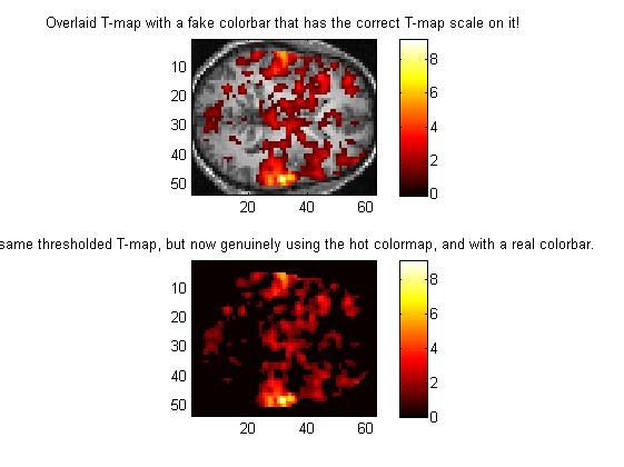
2.7 做对比,那叠加后的解剖图与原始的阈值化的功能图进行比对:
figure(7);
clf;
subplot(2,1,1); %%% Show RGB image and fake colorbar in upper subplot
image(compound_RGB);
axis('image');
% Now set the "colormap" to be hot.
% This won't affect the RGB image at all, because it doesn't use a colormap,
% but it will give us the right colours in the colorbar.
colormap hot;
h = colorbar; %%% h is the handle of the colorbar
%%%% The colorbar actually goes from 1 to 64, but we can label
%%%% it to go from zero to the maximum T-map value.
max_Tmap_value = max(max(Tmap_slice_vals));
desired_colorbar_labels = [ 0 : 2 : max_Tmap_value ];
%%% Start at 0, go up in steps of 2 until we hit the max value
%%%% We can fit these onto the 1-to-64 scale in the same way as we did above
corresponding_values_on_1_to_64_scale = ...
1 + ( 63 * desired_colorbar_labels / max_Tmap_value );
%%%% Now we can use "set" to make the YTick values and labels be what we want:
set(h,'YTick',corresponding_values_on_1_to_64_scale);
set(h,'YTickLabel',desired_colorbar_labels);
title(['Overlaid T-map with a fake colorbar ' ...
'that has the correct T-map scale on it!' ]);
%%%% In the lower subplot, let's show a real colormap plot and a real colorbar,
%%%% so that we can compare them.
subplot(2,1,2); % The lower subplot
imagesc(thresholded_Tmap); % Note that we are using imagesc here, so that
% we use the full range of the REAL colormap
axis('image');
colorbar;
title(['The same thresholded T-map, but now genuinely ' ...
'using the hot colormap, and with a real colorbar.' ]);
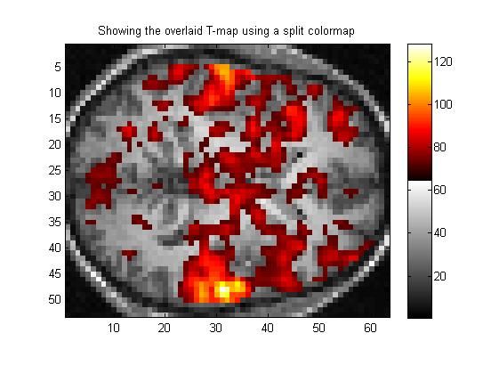
2.8 这里是提供一种替代方案,不用RGB显示,而是将colormap扩大,以容纳更多的颜色:
split_colormap = [ gray_cmap; hot_cmap ];
% So, the first 64 rows are all gray, and any (unscaled) image intensities
% between 1 and 64 will all be coloured from the gray part of the colormap.
% Any image intensities betwen 65 and 128 will be coloured from the hot part.
%
% Above, we already made versions of our anatomical and T-map images
% that were scaled from 1 to 64.
% So, we just need to add another 64 to our T-map image, and
% make an image that has the anatomical's values in places where
% the T-map is below-threshold, and that has the T-maps's values
% in places where the T-map is above-threshold.
Tmap_65_to_128 = 64 + Tmap64; % Tmap64 goes from 1 to 64
image_for_split_colormap = ...
(thresholded_Tmap==0) .* anat64 + ... % Where T-map is below threshold
(thresholded_Tmap>0).* Tmap_65_to_128; % Where T-map is above threshold
figure(8);
clf;
image(image_for_split_colormap);
colormap(split_colormap);
axis('image');
colorbar;
title('Showing the overlaid T-map using a split colormap');
the end 完整代码
%%%% Tutorial on how to show statistical maps overlaid

%%%% on top of anatomical images in Matlab.

%%%% Written by Rajeev Raizada, July 24, 2002.

%%%%

%%%% For a gentle intro to displaying brain images in Matlab,

%%%% look at the program "showing_brain_images_tutorial.m"

%%%%

%%%% Overlaying T-maps on top of anatomical images is

%%%% quite a bit more tricky than simply showing anatomicals,

%%%% so look at the "showing_brain_images_tutorial.m" program

%%%% before this one, if you want a general intro to image displays.

%%%% This program is not intended to be a self-contained intro

%%%% to Matlab and image-displaying.

%%%% For an intro, you should refer to showing_brain_images_tutorial.m

%%%%

%%%% To run either program, you need the file containing the brain images:

%%%% speech_brain_images.mat (2.3Mb)

%%%%

%%%% Please mail any comments or suggestions to: [email protected]


%%%% Often we want to overlay a coloured statistical map

%%%% on top of a grayscale anatomical map.

%%%% If you want a nice, graphical-user-interface based program that

%%%% will do this for you, then check out Matthew Brett's display_slices.m,

%%%% which you can download from:

%%%% http://www.mrc-cbu.cam.ac.uk/Imaging/display_slices.html

%%%%

%%%% The program below shows how you can make such overlays yourself.

%%%% In showing_brain_images_tutorial.m we saw how to use different

%%%% Matlab colormaps. So, you might think that to overlay a T-map

%%%% on top of an anatomical image, we would simply draw the anatomical

%%%% using colormap gray, and then draw the T-map on top of it using

%%%% colormap hot.

%%%% Unfortunately, it isn't quite that easy, because Matlab only lets

%%%% you have one colormap per figure window.

%%%% One way of getting round this obstacle would be to make

%%%% a big compound colormap made up of the gray and hot colormaps

%%%% joined together. That's shown at the end of this program, in Figure 8.

%%%%

%%%% However, a more flexible approach is not to use a colormap at all,

%%%% but instead to specify a real RGB (red-green-blue) colour value

%%%% for every voxel in the image. The main advantage of this

%%%% is that it lets you make the coloured statistical overlay transparent,

%%%% by making a weighted-combination of the anatomical

%%%% and statistical images.

%%%% (In Matlab 6, there is a new way of making images transparent,

%%%% using a new image-property called "alphadata". But the RGB method that

%%%% is shown in this program is more general, and works with Matlab 5 too).

%%%%

%%%% To figure out what RGB values to give, we can read in the RGB values

%%%% from the Matlab colormap matrices. That way, we get to use the

%%%% nice colour-scheme of a pre-made Matlab colormap, without being

%%%% bound by the inflexibility that using a real colormap imposes.

%%%%

%%%% The structure of a Matlab colormap matrix is as follows:

%%%% There are 64 rows, and three columns.

%%%% When we image a matrix unscaled, i.e. using image() instead of imagesc(),

%%%% Matlab takes each matrix-element, sees what whole-number from 1 to 64

%%%% its value is closest to, and looks up the values in that row of the

%%%% colormap matrix. The three values in that row are the RGB values

%%%% for the colour that this element will have when it's drawn in the image.

%%%% E.g. suppose the element has the value 25. Then that element will

%%%% get shown with the RGB values from the 25th row of the colormap matrix.

%%%%

%%%% The trick that we'll use below will be to scale our anatomical and T-map

%%%% images from 1 to 64, then read in the RGB values from the corresponding

%%%% rows of the gray and hot colormap matrices.

%%%%

%%%% Then we'll have an RGB image for the anatomical that will be

%%%% made only of shades of gray, because it will be made from rows

%%%% of the gray colormap matrix. And we'll have an RGB image for the T-map

%%%% that will be made out of rows from the hot colormap matrix.

%%%%

%%%% Then we can make a weighted sum of these two images and display it.


%%%%%%% First, load in the file containing the brain images

load speech_brain_images.mat


%%%% Let's look at the 18th axial slice.

%%%% This goes through Heschl's gyrus, which is auditory cortex


axial_slice_number = 18;


%%%% Read the values from the 3D matrix subj_3danat

anat_slice_vals = subj_3danat(:,:,axial_slice_number);


%%%% Use squeeze to get rid of any redundant 3rd dimension that

%%%% might be left over. This is described in

%%%% more detail in showing_brain_images_tutorial.m


anat_slice_2D = squeeze(anat_slice_vals);


%%%% In order to make it easier for us to match up the

%%%% anatomical values to the 64-entries in Matlab's standard

%%%% gray colormap, we're going to scale the anatomical image

%%%% values so that they are all integers going from 1 to 64


%%%% First scale it from 0 to 1 by dividing by the maximum value.

%%%% Because it's a 2D matrix, we have to perform the max() operation

%%%% twice, once for each dimension. Then we end up with one max value,

%%%% which we can use as a divisor.


anat01 = anat_slice_2D ./ max(max(anat_slice_2D));


%%%% Next, multiply by 63 and round to the nearest whole number

anat0_63 = round( 63 * anat01 );


%%%% Finally, add 1, in order to make a matrix that goes from 1 to 64


anat64 = anat0_63 + 1;


%%%%%%%%%%%% Now let's do the same for the thresholded T-map


Tmap_slice_vals = speech_Tmap(:,:,axial_slice_number);


Tmap_slice_2D = squeeze(Tmap_slice_vals);


T_threshold = 1;    %%% Let's pick a fairly low threshold, because it helps

                    %%% for showing the effect of transparent overlay later.


%%%% To threshold the map, make a logical 0/1 matrix that says

%%%% whether each voxel is above-threshold or not, and multiply

%%%% it element-by-element by the raw T-map values.

%%%% This is explained in a more step-by-step way

%%%% in the companion program showing_brain_images_tutorial.m


thresholded_Tmap = ( Tmap_slice_2D > T_threshold ) .* Tmap_slice_2D;


Tmap01 = thresholded_Tmap ./ max(max(thresholded_Tmap));


Tmap0_63 = round( 63 * Tmap01 );


Tmap64 = 1 + Tmap0_63;


%%%%%%%%%%%%%%%%%%%%%%%%%%%%%%%%%%%%%%%%%%%%%%%%%%%%%%%%%%%%%%%%

% Ok, now we have made two matrices scaled from 1 to 64,

% one for the anatomical image, and the other for the T-map image

%

% The next step is to make a full RGB-image for each image,

% by looking up the corresponding rows of the gray and hot colormaps.

%

% An RGB-image is a 3D-matrix.

% It has three "colour slabs" that are joined up along the third dimension.

% The first slab is an image full of Red values.

% The second slab is an image full of Green values.

% And the third slab is an image of Blue values.


% First make 3D matrices full of zeros, to hold the values

% that we are about to create for the anatomical and T-map RGB images.

% These have three slabs in the 3rd dimension, and are the same size as

% the anatomical and the Tmap matrices in the first two dimensions.


anat_RGB = zeros(size(anat64,1), size(anat64,2), 3);

                    %%% This will hold the anatomical image's RBG values


Tmap_RGB = zeros(size(Tmap64,1), size(Tmap64,2), 3);

                    %%% This will hold the T-map image's RBG values


%%% Now, let's get hold of copies of Matlab's gray and hot

%%% colormap matrices. As far as I know, we need to make a figure

%%% first in order to do this. That's fine, because we want to

%%% look at our newly created 1-to-64 scaled images anyway.


figure(1);

clf;

image(anat64);  %%% Note that this is image(), not imagesc() !!!

                %%% This looks the same as if we had used imagesc,

                %%% because the image values are *already* scaled

                %%% to cover the whole colormap, from black to white

colormap gray;

axis('image');

colorbar;

title('The anatomical image after we have scaled it from 1 to 64');


% Now that we are in colormap gray, let's make a copy of the colormap matrix


gray_cmap = colormap;   %%% This reads in the current colormap matrix


%%%%%%%% Now let's do the same for the hot colormap


figure(2);

clf;

image(Tmap64);  %%% Again, note that we are using image(), not imagesc()

colormap hot;

axis('image');

colorbar;

title('The T-map image after we have scaled it from 1 to 64');


%%%%% Make a copy of the new current colormap matrix, which is now hot.

hot_cmap = colormap;


%%%%%%%%%%%%%%%%%%%%%%%%%%%%%%%%%%%%%%%%%%%%%%%%%%%%%%%%%%%%%%%%

%

% Ok, now we have copies of the gray and hot colormap matrices,

% with their 64 rows each, we have anatomical and T-map images scaled

% from 1 to 64, so that we can match each value to a colormap matrix row,

% and we have empty place-holder matrices to store the looked-up RGB values.

% So, we're ready to look-up and store the appropriate RGB values.


for RGB_dim = 1:3,  %%% Loop through the three slabs: R, G, and B


    %%% Each entry in each 1-to-64-scaled matrix gives us a row

    %%% in the colormap matrix to go look-up.

    %%% That row has three columns: the R, G and B values for that colour.

    gray_cmap_rows_for_anat = anat64;

    hot_cmap_rows_for_Tmap = Tmap64;


    %%% We'll read in one of these R, G, or B values at a time,

    %%% depending on which colour-slab we're building.

    %%% The colormap entry we want is in the RGB_dim-th column,

    %%% and in the row that we determined above.

    %%% Note that we're actually looking up all the rows at once,

    %%% because we're giving Matlab an entire matrix in the row-position.


    colour_slab_vals_for_anat = gray_cmap(gray_cmap_rows_for_anat, RGB_dim);

    colour_slab_vals_for_Tmap = hot_cmap(hot_cmap_rows_for_Tmap, RGB_dim);


    %%%% These colour-slab values turn out to be in column vector format,

    %%%% and need to be reshaped into being the same size as image matrices.


    anat_RGB(:,:,RGB_dim) = reshape( colour_slab_vals_for_anat, size(anat64));

    Tmap_RGB(:,:,RGB_dim) = reshape( colour_slab_vals_for_Tmap, size(Tmap64));


end;  % End of loop through the RGB dimension.


%%%% Now that we've made our RGB images, let's look at them

%%%% Note that these types of images do *not* have colormaps.

%%%% Every image pixel has three numbers attached to it, not just one,

%%%% and those three numbers define the colour for that pixel directly,

%%%% by giving its R, G and B values.


figure(3);

clf;

image(anat_RGB);

axis('image');

title('The anatomical RGB image, with no colormap')


figure(4);

clf;

image(Tmap_RGB);

axis('image');

title('The T-map RGB image, with no colormap')


% You might be thinking: my RGB images in Figs.3 and 4

% look exactly like my colormap images in Fig.1 and 2 !!

% Why did I go to all that work just to make images that end up

% looking exactly the same as the ones I started with ?


% The answer is that now we can make a compound image that is

% a mixture of the anatomical image and the T-map transparently

% overlaid on top of it.

%

% We achieve the transparency by taking a weighted sum of the

% anatomical image and the T-map image.

% The more weighting we give to the T-map, the more opaque it will look

% when we overlay it on top of the anatomical.


% Let's make the opacity range from 0 to 1, with 0 being fully transparent.


Tmap_opacity = 0.4;     % 0.4 is a reasonable opacity value to try first


%%%% Make a place-holder matrix to hold the compound weighted-sum image


compound_RGB = zeros(size(anat64,1), size(anat64,2), 3);

                    %%% The anat and the T-map are the same size,

                    %%% we could have chosen either.


%%% Now build up the compound image, one colour-slab at a time, like above.

%%% Where the T-map is below threshold, we only want the anatomical's values.

%%% Where the T-map is above-threshold, we want a weighted sum

%%% of the T-map RGB values and the anatomical's RGB values.


for RGB_dim = 1:3,  %%% Loop through the three slabs: R, G, and B


    compound_RGB(:,:,RGB_dim) = ...

        (thresholded_Tmap==0) .* ...    % Where T-map is below threshold

            anat_RGB(:,:,RGB_dim) + ...

        (thresholded_Tmap>0).* ...      % Where T-map is above threshold

            ( (1-Tmap_opacity) * anat_RGB(:,:,RGB_dim) + ...

               Tmap_opacity * Tmap_RGB(:,:,RGB_dim) );

                        % Opacity-weighted sum of anatomical and T-map

end;


%%%% Before displaying our newly-made compound image,

%%%% we have to make sure that none of the RGB values exceeds 1.


compound_RGB = min(compound_RGB,1);


%%%% Now let's look at the fruit of our labours!


figure(5);

clf;

image(compound_RGB);

axis('image');

title('The T-map transparently overlaid on the anatomical')


%%%% To look at the effect of varying the opacity, let's try a few values


figure(6);

clf;


for i = 1:4,


    Tmap_opacity = 0.25*i;   % This will give opacities: 0.25, 0.5, 0.75, 1


    %%%%%%%% Go through a copy of the loop above to make a new compound image


    for RGB_dim = 1:3,  %%% Loop through the three slabs: R, G, and B


        compound_RGB(:,:,RGB_dim) = ...

        (thresholded_Tmap==0) .* ...    % Where T-map is below threshold

            anat_RGB(:,:,RGB_dim) + ...

        (thresholded_Tmap>0).* ...      % Where T-map is above threshold

            ( (1-Tmap_opacity) * anat_RGB(:,:,RGB_dim) + ...

               Tmap_opacity * Tmap_RGB(:,:,RGB_dim) );

                        % Opacity-weighted sum of anatomical and T-map

    end;

    compound_RGB = min(compound_RGB,1);


    %%%%%%%% Plot the new compound image

    subplot(2,2,i);

    image(compound_RGB);

    axis('image');

    title(['T-map opacity = ' num2str(Tmap_opacity) ]);


end;    %%% End of loop through i


%%%%%%%%% Even though these RGB images don't have colormaps,

%%%%%%%%% we can make a fake colorbar showing the real T-map values.

%%%%%%%%% We'll make a colorbar, then use "set" and "get" to manipulate it.


% Let's have two subplots.

% In the upper subplot, we'll manufacture a fake colorbar

% that will show the the real T-map scaling.

%

% In the lower subplot, we'll show a real colorbar,

% so that we can check that they look the same


figure(7);

clf;

subplot(2,1,1);         %%% Show RGB image and fake colorbar in upper subplot

image(compound_RGB);

axis('image');


% Now set the "colormap" to be hot.

% This won't affect the RGB image at all, because it doesn't use a colormap,

% but it will give us the right colours in the colorbar.


colormap hot;

h = colorbar;   %%% h is the handle of the colorbar


%%%% The colorbar actually goes from 1 to 64, but we can label

%%%% it to go from zero to the maximum T-map value.


max_Tmap_value = max(max(Tmap_slice_vals));


desired_colorbar_labels = [ 0 : 2 : max_Tmap_value ];

        %%% Start at 0, go up in steps of 2 until we hit the max value


%%%% We can fit these onto the 1-to-64 scale in the same way as we did above


corresponding_values_on_1_to_64_scale = ...

    1 +  ( 63 * desired_colorbar_labels / max_Tmap_value );


%%%% Now we can use "set" to make the YTick values and labels be what we want:


set(h,'YTick',corresponding_values_on_1_to_64_scale);

set(h,'YTickLabel',desired_colorbar_labels);


title(['Overlaid T-map with a fake colorbar ' ...

       'that has the correct T-map scale on it!' ]);


%%%% In the lower subplot, let's show a real colormap plot and a real colorbar,

%%%% so that we can compare them.


subplot(2,1,2);             % The lower subplot

imagesc(thresholded_Tmap);  % Note that we are using imagesc here, so that

                            % we use the full range of the REAL colormap

axis('image');

colorbar;


title(['The same thresholded T-map, but now genuinely ' ...

       'using the hot colormap, and with a real colorbar.' ]);


%%%%%%%%%%%%%%%%%%%%%%%%%%%%%%%%%%%%%%%%%%%%%%%%%%%%%%%%%%%%%%%%%%%%%%%%%%%%

%

% Finally, let's try using a "split colormap".

% This is simpler than the RGB approach, but can't give transparent overlays.

%

% To use a split colormap, we make a new 128-row colormap matrix

% by stacking the gray colormap on top of the hot colormap.

% Note that we already made matrices holding these two colormaps, above.

% We called the matrices gray_cmap and hot_cmap.


split_colormap = [ gray_cmap; hot_cmap ];


% So, the first 64 rows are all gray, and any (unscaled) image intensities

% between 1 and 64 will all be coloured from the gray part of the colormap.

% Any image intensities betwen 65 and 128 will be coloured from the hot part.

%

% Above, we already made versions of our anatomical and T-map images

% that were scaled from 1 to 64.

% So, we just need to add another 64 to our T-map image, and

% make an image that has the anatomical's values in places where

% the T-map is below-threshold, and that has the T-maps's values

% in places where the T-map is above-threshold.


Tmap_65_to_128 = 64 + Tmap64;   % Tmap64 goes from 1 to 64


image_for_split_colormap = ...

    (thresholded_Tmap==0) .* anat64  + ...  % Where T-map is below threshold

    (thresholded_Tmap>0).* Tmap_65_to_128;  % Where T-map is above threshold


figure(8);

clf;

image(image_for_split_colormap);

colormap(split_colormap);

axis('image');

colorbar;

title('Showing the overlaid T-map using a split colormap');