线性回归的N种姿势

1. Naive Solution

We want to find x̂  x ^ that minimizes:

∣∣∣∣Ax̂ −b∣∣∣∣2 | | A x ^ − b | | 2

Another way to think about this is that we are interested in where vector b b ​ is closest to the subspace spanned by A A ​ (called the range of A A ​ ). Ax̂  A x ^ ​ is the projection of b b ​ onto A A ​ . Since b−Ax̂  b − A x ^ ​ must be perpendicular to the subspace spanned by A A ​ , we see that

AT(b−Ax̂ )=0 A T ( b − A x ^ ) = 0

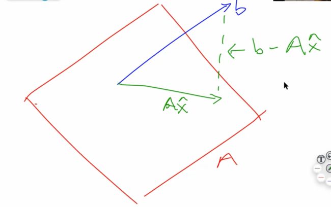
(we are using AT A T because we want to multiply each column of A A by b−Ax̂  b − A x ^

This leads us to the normal equations:

x=(ATA)−1ATb x = ( A T A ) − 1 A T b

但是这种方法不是很practical，因为要求矩阵的逆，比较麻烦。

def ls_naive(A, b):
    # not practical，因为直接求了矩阵的逆，很麻烦
     return np.linalg.inv(A.T @ A) @ A.T @ b

coeffs_naive = ls_naive(trn_int, y_trn)
regr_metrics(y_test, test_int @ coeffs_naive)

2. Cholesky Factorization

Normal equations:

ATAx=ATb A T A x = A T b

If A A has full rank, the pseudo-inverse (ATA)−1AT ( A T A ) − 1 A T is a square, hermitian positive definite matrix.

【注意】Cholesky一定要是正定矩阵！虽然这个操作又快又好，但是使用场景有限！

The standard way of solving such a system is Cholesky Factorization, which finds upper-triangular R such that ATA=RTR A T A = R T R . ( RT R T is lower-triangular )

AtA = A.T @ A
Atb = A.T @ b

R = scipy.linalg.cholesky(AtA)

# check our factorization
np.linalg.norm(AtA - R.T @ R)

Q：为啥变成 RTRx=ATb R T R x = A T b 会变简单？

之前提过，上三角矩阵解线性方程组时会简单许多（最后一行只有一个未知数）。

所以先求 RTw=ATb R T w = A T b 再求 Rx=w R x = w 会easier。

ATAx=ATbRTRx=ATbRTw=ATbRx=w A T A x = A T b R T R x = A T b R T w = A T b R x = w

def ls_chol(A, b):
    R = scipy.linalg.cholesky(A.T @ A)
    w = scipy.linalg.solve_triangular(R, A.T @ b, trans='T')
    return scipy.linalg.solve_triangular(R, w)

%timeit coeffs_chol = ls_chol(trn_int, y_trn)

3. QR Factorization

Q Q is orthonormal, R R is upper-triangular.

Ax=bA=QRQRx=bQ−1=QTQTQRx=QTbRx=QTb A x = b A = Q R Q R x = b Q − 1 = Q T Q T Q R x = Q T b R x = Q T b

Then once again, Rx R x is easier to solve than Ax A x .

def ls_qr(A,b):
    Q, R = scipy.linalg.qr(A, mode='economic')
    return scipy.linalg.solve_triangular(R, Q.T @ b)

coeffs_qr = ls_qr(trn_int, y_trn)
regr_metrics(y_test, test_int @ coeffs_qr)

4. SVD

都是同样的问题，要求 x x 。 U U 的column orthonormal， ∑ ∑ 是对角阵， V V 是row orthonormal.

Ax=bA=UΣVΣVx=UTbΣw=UTbx=VTw A x = b A = U Σ V Σ V x = U T b Σ w = U T b x = V T w

解 Σw=UTb Σ w = U T b 甚至比上三角矩阵 R R 更简单（每行只有一个未知量）。然后 Vx=w V x = w 又可以直接用orthonormal的性质，直接等于 VTw V T w 。

SVD gives the pseudo-inverse.

def ls_svd(A,b):
    m, n = A.shape
    U, sigma, Vh = scipy.linalg.svd(A, full_matrices=False, lapack_driver='gesdd')
    w = (U.T @ b)/ sigma
    return Vh.T @ w

coeffs_svd = ls_svd(trn_int, y_trn)
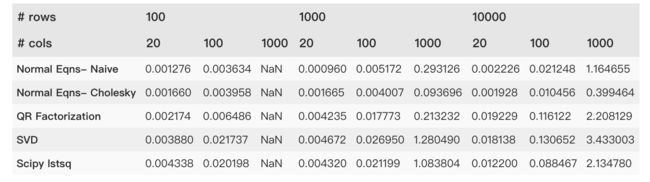
regr_metrics(y_test, test_int @ coeffs_svd)

5. Timing Comparison

Matrix Inversion: 2n3 2 n 3

Matrix Multiplication: n3 n 3

Cholesky: 13n3 1 3 n 3

QR, Gram Schmidt: 2mn2 2 m n 2 , m≥n m ≥ n (chapter 8 of Trefethen)

QR, Householder: 2mn2−23n3 2 m n 2 − 2 3 n 3 (chapter 10 of Trefethen)

Solving a triangular system: n2 n 2

Why Cholesky Factorization is Fast:

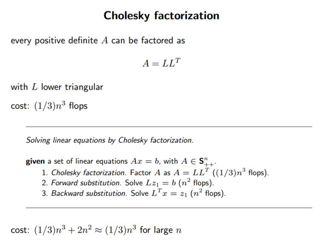
(source: Stanford Convex Optimization: Numerical Linear Algebra Background Slides)