Coursera-Machine-Learning-ex4
上一个练习中我们使用给定的权重矩阵对手写数字进行预测,本次练习中,我们尝试去学习参数θ。
Neural Networks
首先使用displayData方法对训练集数据进行可视化。

和之前的训练集一样,共5000个训练样本,每个样本为20*20像素的图片,展开以400维向量形式给出。训练样本处理如下:

首先确定结构,我们本次使用三层结构,一个输入层,一个隐藏层,一个输出层。由于我们每个样本输入有400个元素,所以我们设定400个输入单元(不计算偏置单元),那么我们需要θ1和θ2两个权重矩阵需要学习,其中隐藏层有25个单元,输出层有10个单元。

然后我们首先完成代价函数和梯度下降计算部分。首先利用公式写出h(x)的计算结果,写出不含正则项的代价函数。
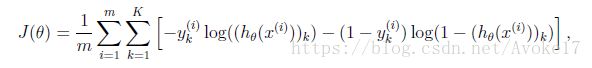
经过程序验证后可以加入正则项,公式如下:

然后我们需要使用反向传播算法写出偏导项的计算公式,反向传播算法和nnCostFunction.m代码如下:

function [J grad] = nnCostFunction(nn_params, ...
                                   input_layer_size, ...
                                   hidden_layer_size, ...
                                   num_labels, ...
                                   X, y, lambda)
%NNCOSTFUNCTION Implements the neural network cost function for a two layer
%neural network which performs classification
%   [J grad] = NNCOSTFUNCTON(nn_params, hidden_layer_size, num_labels, ...
%   X, y, lambda) computes the cost and gradient of the neural network. The
%   parameters for the neural network are "unrolled" into the vector
%   nn_params and need to be converted back into the weight matrices.
%
%   The returned parameter grad should be a "unrolled" vector of the
%   partial derivatives of the neural network.
%

% Reshape nn_params back into the parameters Theta1 and Theta2, the weight matrices
% for our 2 layer neural network
Theta1 = reshape(nn_params(1:hidden_layer_size * (input_layer_size + 1)), ...
                 hidden_layer_size, (input_layer_size + 1));

Theta2 = reshape(nn_params((1 + (hidden_layer_size * (input_layer_size + 1))):end), ...
                 num_labels, (hidden_layer_size + 1));

% Setup some useful variables
m = size(X, 1);

% You need to return the following variables correctly
J = 0;
Theta1_grad = zeros(size(Theta1));
Theta2_grad = zeros(size(Theta2));

% ====================== YOUR CODE HERE ======================
% Instructions: You should complete the code by working through the
%               following parts.
%
% Part 1: Feedforward the neural network and return the cost in the
%         variable J. After implementing Part 1, you can verify that your
%         cost function computation is correct by verifying the cost
%         computed in ex4.m
%
% Part 2: Implement the backpropagation algorithm to compute the gradients
%         Theta1_grad and Theta2_grad. You should return the partial derivatives of
%         the cost function with respect to Theta1 and Theta2 in Theta1_grad and
%         Theta2_grad, respectively. After implementing Part 2, you can check
%         that your implementation is correct by running checkNNGradients
%
%         Note: The vector y passed into the function is a vector of labels
%               containing values from 1..K. You need to map this vector into a
%               binary vector of 1's and 0's to be used with the neural network
%               cost function.
%
%         Hint: We recommend implementing backpropagation using a for-loop
%               over the training examples if you are implementing it for the
%               first time.
%
% Part 3: Implement regularization with the cost function and gradients.
%
%         Hint: You can implement this around the code for
%               backpropagation. That is, you can compute the gradients for
%               the regularization separately and then add them to Theta1_grad
%               and Theta2_grad from Part 2.
%

a1 = [ones(m, 1) X];
z2 = a1 * Theta1';
a2 = sigmoid(z2);
a2 = [ones(m, 1) a2];
z3 = a2 * Theta2';
h = sigmoid(z3);

yk = zeros(m, num_labels);
for i = 1:m
    yk(i, y(i)) = 1;
end
J = (1/m)* sum(sum(((-yk) .* log(h) - (1 - yk) .* log(1 - h))));


r = (lambda / (2 * m)) * (sum(sum(Theta1(:, 2:end) .^ 2))
    + sum(sum(Theta2(:, 2:end) .^ 2)));
J = J + r;

for row = 1:m
    a1 = [1 X(row,:)]';
    z2 = Theta1 * a1;
    a2 = sigmoid(z2);
    a2 = [1; a2];
    z3 = Theta2 * a2;
    a3 = sigmoid(z3);

    z2 = [1; z2];
    delta3 = a3 - yk'(:, row);
    delta2 = (Theta2' * delta3) .* sigmoidGradient(z2);
    delta2 = delta2(2:end);

    Theta1_grad = Theta1_grad + delta2 * a1';
    Theta2_grad = Theta2_grad + delta3 * a2';

end

Theta1_grad = Theta1_grad ./ m;
Theta1_grad(:, 2:end) = Theta1_grad(:, 2:end) ...
        + (lambda/m) * Theta1(:, 2:end);
Theta2_grad = Theta2_grad ./ m;
Theta2_grad(:, 2:end) = Theta2_grad(:, 2:end) + ...
        + (lambda/m) * Theta2(:, 2:end);
% -------------------------------------------------------------

% =========================================================================

% Unroll gradients
grad = [Theta1_grad(:) ; Theta2_grad(:)];
end进行神经网络训练时,权重矩阵的随机初始化很重要。这里我们设置初始化的随机值在-0.12至0.12之间,设定一个较小的值以确保证学习过程更有效率。randInitializeWeights.m的代码如下:
function W = randInitializeWeights(L_in, L_out)
%RANDINITIALIZEWEIGHTS Randomly initialize the weights of a layer with L_in
%incoming connections and L_out outgoing connections
%   W = RANDINITIALIZEWEIGHTS(L_in, L_out) randomly initializes the weights
%   of a layer with L_in incoming connections and L_out outgoing
%   connections.
%
%   Note that W should be set to a matrix of size(L_out, 1 + L_in) as
%   the first column of W handles the "bias" terms
%

% You need to return the following variables correctly
W = zeros(L_out, 1 + L_in);

% ====================== YOUR CODE HERE ======================
% Instructions: Initialize W randomly so that we break the symmetry while
%               training the neural network.
%
% Note: The first column of W corresponds to the parameters for the bias unit
%

epsilon_init=0.12;
W=rand(L_out,1+L_in)*2*epsilon_init-epsilon_init;

% =========================================================================

end然后我们加入梯度验证,使用近似项计算偏导项值,checkNNGradients.m代码如下:
function numgrad = computeNumericalGradient(J, theta)
%COMPUTENUMERICALGRADIENT Computes the gradient using "finite differences"
%and gives us a numerical estimate of the gradient.
%   numgrad = COMPUTENUMERICALGRADIENT(J, theta) computes the numerical
%   gradient of the function J around theta. Calling y = J(theta) should
%   return the function value at theta.

% Notes: The following code implements numerical gradient checking, and
%        returns the numerical gradient.It sets numgrad(i) to (a numerical
%        approximation of) the partial derivative of J with respect to the
%        i-th input argument, evaluated at theta. (i.e., numgrad(i) should
%        be the (approximately) the partial derivative of J with respect
%        to theta(i).)
%

numgrad = zeros(size(theta));
perturb = zeros(size(theta));
e = 1e-4;
for p = 1:numel(theta)
    % Set perturbation vector
    perturb(p) = e;
    loss1 = J(theta - perturb);
    loss2 = J(theta + perturb);
    % Compute Numerical Gradient
    numgrad(p) = (loss2 - loss1) / (2*e);
    perturb(p) = 0;
end

end
一旦计算出的值和近似值之差很小,我们就可以确认梯度计算是正确的。关闭梯度检验,然后我们使用fmincg来学习参数θ,便可以得到使代价函数最小的参数。