07_Ensemble Learning and Random Forests_02_AdaBoost_Gradient Boosting_XGBoost

voting_clf.score(X_val, y_val)

AdaBoost

https://blog.csdn.net/Linli522362242/article/details/104771157

Gradient Boosting梯度提升

     Another very popular Boosting algorithm is Gradient Boosting. Just like AdaBoost, Gradient Boosting works by sequentially adding predictors to an ensemble, each one correcting its predecessor. However, instead of tweaking the instance weights at every iteration like AdaBoost does, this method tries to fit the new predictor to the residual errors made by the previous predictor.

     Let's go through a simple regression example using Decision Trees as the base predictors (of course Gradient Boosting also works great with regression tasks). This is called Gradient Tree Boosting, or Gradient Boosted Regression Trees (GBRT).

First, let's fit a DecisionTreeRegressor to the training set (for example, a noisy quadratic training set):

np.random.seed(42)
X = np.random.rand(100,1) - 0.5
y = 3*X[:,0]**2 + 0.05*np.random.randn(100)

from sklearn.tree import DecisionTreeRegressor

tree_reg1 = DecisionTreeRegressor(max_depth=2, random_state=42)
tree_reg1.fit(X,y)

Now train a second DecisionTreeRegressor on the residual errors made by the first predictor:

y2 = y-tree_reg1.predict(X) #residual errors
tree_reg2 = DecisionTreeRegressor(max_depth=2, random_state=42)
tree_reg2.fit(X,y2) #y-tree_reg1.predict(X)

Then we train a third regressor on the residual errors made by the second predictor:

y3 = y2-tree_reg2.predict(X)
tree_reg3 = DecisionTreeRegressor(max_depth=2, random_state=42)
tree_reg3.fit(X,y3)

Now we have an ensemble containing three trees. It can make predictions on a new instance simply by adding up the predictions of all the trees:

X_new = np.array([[0.8]])

y_pred = sum( tree.predict(X_new) for tree in (tree_reg1, tree_reg2, tree_reg3) )
y_pred

def plot_predictions(regressors, X,y, axes, label=None, style="r-", data_style="b.", data_label=None):
    x1 = np.linspace(axes[0], axes[1], 500)
    y_pred = sum( regressor.predict( x1.reshape(-1,1) ) for regressor in regressors )
    plt.plot( X[:,0], y, data_style, label=data_label )      # plotting data points
    plt.plot( x1, y_pred, style, linewidth=2, label=label )  # plotting decision boundaries 
    if label or data_label:
        plt.legend( loc="upper center", fontsize=16 )
    plt.axis(axes)

plt.figure( figsize=(13,13) )

plt.subplot(321)
plot_predictions( [tree_reg1], X,y, axes=[ -0.5,0.5, -0.1,0.8 ], label="$h_1(x_1)$", style="g-", 
                 data_label="Training set")
plt.ylabel( "$y$", fontsize=16, rotation=0 )#IndexError: string index out of range: plt.ylabel("$y_$", fontsize=16, rotation=0)
plt.title( "Residuals and tree predictions", fontsize=16 )

plt.subplot(322)
plot_predictions( [tree_reg1], X,y, axes=[ -0.5,0.5, -0.1,0.8 ], label="$h(x_1)=h_1(x_1)$", 
                 data_label="Training set")
plt.ylabel("y^ ", fontsize=16, rotation=0)
plt.title("Ensemble predictions", fontsize=16)


plt.subplot(323)
plot_predictions( [tree_reg2], X,y2, axes=[ -0.5,0.5, -0.5,0.5 ], label="$h_2(x_1)$", style="g-", 
                 data_label="Residuals", data_style="k+") #y2 = y-tree_reg1.predict(X) #residual errors
plt.ylabel("$y-h_1(x_1)$", fontsize=16, rotation=0)

plt.subplot(324)
plot_predictions( [tree_reg1,tree_reg2], X,y, axes=[ -0.5,0.5, -0.1,0.8 ], label="$h(x_1)=h_1(x_1)+h_2(x_1)$")
plt.ylabel("y^ ", fontsize=16, rotation=0)


plt.subplot(325)
plot_predictions( [tree_reg3], X,y3, axes=[-0.5,0.5, -0.5,0.5], label="$h_3(x_1)$", style="g-", 
                 data_label="$y-h_1(x_1)-h_2(x_1)$", data_style="k+") #y3 = y-tree_reg2.predict(X)
plt.ylabel("$y-h_1(x_1)-h_2(x_1)$", fontsize=16)
plt.xlabel("$x_1$", fontsize=16)

plt.subplot(326)
plot_predictions( [tree_reg1, tree_reg2, tree_reg3], X,y, axes=[-0.5,0.5, -0.1,0.8], 
                 label="$h(x_1)=h_1(x_1)+h_2(x_1)+h_3(x_1)$" )
plt.xlabel("$x_1$", fontsize=16)
plt.ylabel("y^", fontsize=16, rotation=0)

plt.subplots_adjust(left=0.1, right=0.9, wspace=0.25)
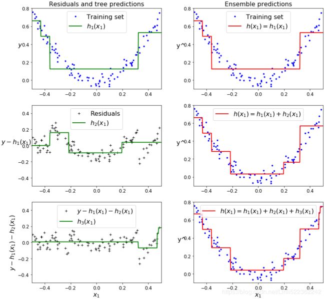
plt.show()

Figure 7-9. Gradient Boosting

     Figure 7-9 represents the predictions of these three trees in the left column, and the ensemble's predictions in the right column. In the first row, the ensemble has just one tree, so its predictions are exactly the same as the first tree's predictions. In the second row, a new tree is trained on the residual errors of the first tree. On the right you can see that the ensemble's predictions are equal to the sum of the predictions of the first two trees. Similarly, in the third row another tree is trained on the residual errors of the second tree. You can see that the ensemble's predictions gradually get better as trees are added to the ensemble.

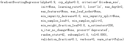
     A simpler way to train GBRT ensembles is to use Scikit-Learn’s GradientBoostingRegressor class. Much like the RandomForestRegressor class, it has hyperparameters to control the growth of Decision Trees (e.g., max_depth, min_samples_leaf, and so on), as well as hyperparameters to control the ensemble training, such as the number of trees (n_estimators). The following code creates the same ensemble as the previous one:

from sklearn.ensemble import GradientBoostingRegressor
                                                            ###
gbrt = GradientBoostingRegressor( max_depth=2, n_estimators=3, learning_rate=0.1, random_state=42 )
gbrt.fit( X,y )

                                                                 ###
gbrt_slow = GradientBoostingRegressor( max_depth=2, n_estimators=200, learning_rate=0.1, random_state=42 )
gbrt_slow.fit( X,y )

fix, axes = plt.subplots( ncols=2, figsize=(10,4), sharey=True )

plt.sca( axes[0] )
plot_predictions( [gbrt], X,y, axes=[ -0.5,0.5, -0.1,0.8 ], label="Ensemble predictions" )
plt.title( "learning_rate={}, n_estimators={}".format( gbrt.learning_rate, gbrt.n_estimators ), fontsize=14 )
plt.xlabel( "$x_1$", fontsize=16 )
plt.ylabel( "$y$", fontsize=16, rotation=0 )

plt.sca( axes[1] )
plot_predictions( [gbrt_slow], X,y, axes=[ -0.5,0.5, -0.1,0.8 ], label="Ensemble predictions" )
plt.title( "learning_rate={}, n_estimators={}".format( gbrt_slow.learning_rate, gbrt_slow.n_estimators ), fontsize=14)
plt.xlabel( "$x_1$", fontsize=16 )

plt.show()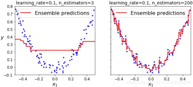

Figure 7-10. GBRT ensembles with not enough predictors (left) and too many (right)

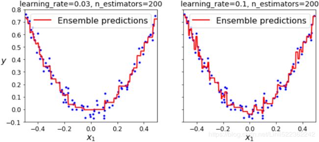
     The learning_rate hyperparameter scales the contribution of each tree. If you set it to a low value, such as 0.1, you will need more trees in the ensemble to fit the training set, but the predictions will usually generalize better. This is a regularization technique called shrinkage收缩. Figure 7-10 shows two GBRT ensembles trained with a low learning rate: the one on the left does not have enough trees to fit the training set, while the one on the right has too many trees and overfits the training set.

     In order to find the optimal number of trees, you can use early stopping (see https://blog.csdn.net/Linli522362242/article/details/104070847). A simple way to implement this is to use the staged_predict() method: it returns an iterator over the predictions made by the ensemble at each stage of training
(with one tree, two trees, etc.). The following code trains a GBRT ensemble with 120 trees, then measures the validation error at each stage of training to find the optimal number of trees, and finally trains another GBRT ensemble using the optimal number of trees:

import numpy as np
from sklearn.model_selection import train_test_split
from sklearn.metrics import mean_squared_error

X_train, X_val, y_train, y_val = train_test_split( X,y, random_state=49 )

gbrt = GradientBoostingRegressor( max_depth=2, n_estimators=120, random_state=42 )
gbrt.fit( X_train, y_train )

errors = [ mean_squared_error(y_val, y_pred) for y_pred in gbrt.staged_predict(X_val) ]
best_n_estimators = np.argmin(errors) + 1# best_n_estimators=index+1=55+1

gbrt_best = GradientBoostingRegressor( max_depth=2, n_estimators=best_n_estimators, random_state=42 )
gbrt_best.fit( X_train, y_train )

min_error = np.min(errors)
min_error

def plot_predictions(regressors, X,y, axes, label=None, style="r-", data_style="b.", data_label=None):
    x1 = np.linspace(axes[0], axes[1], 500)
    y_pred = sum( regressor.predict( x1.reshape(-1,1) ) for regressor in regressors )
    plt.plot( X[:,0], y, data_style, label=data_label )      # plotting data points
    plt.plot( x1, y_pred, style, linewidth=2, label=label )  # plotting decision boundaries 
    if label or data_label:
        plt.legend( loc="upper center", fontsize=16 )
    plt.axis(axes)

plt.figure( figsize=(10,4) )

plt.subplot(121)
plt.plot( errors, "b.-" ) #plotting error curve
plt.plot( [best_n_estimators, best_n_estimators], [0,min_error], "k--" ) # vertical 
plt.plot( [0,120], [min_error, min_error], "k--" ) # tangent line        #horizontal
plt.plot( best_n_estimators, min_error, "ko" ) #minimum error point
plt.axis([ 0,120, 0,0.01 ])
plt.xlabel("Number of trees")
plt.ylabel("Error", fontsize=16)
plt.title("Valication error", fontsize=14)

plt.subplot(122)
plot_predictions( [gbrt_best], X,y, axes=[ -0.5,0.5, -0.1,0.8 ] )
plt.title( "Best model (%d trees)" % best_n_estimators, fontsize=14 )
plt.ylabel( "$y$", fontsize=16, rotation=0 )
plt.xlabel( "$x_1$", fontsize=16)

plt.show()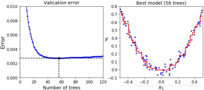

Figure 7-11. Tuning the number of trees using early stopping

     The validation errors are represented on the left of Figure 7-11, and the best model's predictions are represented on the right.

     It is also possible to implement early stopping by actually stopping training early (instead of training a large number of trees first and then looking back to find the optimal number). You can do so by setting warm_start=True, which makes Scikit-Learn keep existing trees when the fit() method is called, allowing incremental training允许增量训练. The following code stops training when the validation error does not improve for five iterations in a row:

gbrt = GradientBoostingRegressor( max_depth=2, warm_start=True, random_state=42 )

min_val_error = float( "inf" )
error_going_up = 0 
for n_estimators in range(1,120):
    gbrt.n_estimators = n_estimators
    gbrt.fit(X_train, y_train)
    y_pred = gbrt.predict( X_val )
    val_error = mean_squared_error(y_val, y_pred)
    if val_error < min_val_error:
        min_val_error=val_error
        error_going_up = 0
    else:
        error_going_up +=1
        if error_going_up == 5:
            break # early stopping

print(gbrt.n_estimators)

print("Minimum validation MSE:", min_val_error)

     The GradientBoostingRegressor class also supports a subsample hyperparameter, which specifies the fraction of training instances to be used for training each tree. For example, if subsample=0.25, then each tree is trained on 25% of the training instances, selected randomly. As you can probably guess by now, this trades a higher bias for a lower variance. It also speeds up training considerably. This technique is called Stochastic Gradient Boosting.

######################################
NOTE
It is possible to use Gradient Boosting with other cost functions. This is controlled by the loss hyperparameter (see Scikit-
Learn's documentation for more details).
######################################

Using XGBoost

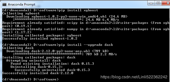
import xgboost

 AttributeError: module 'pandas.core.computation' has no attribute 'expressions'

https://xgboost.readthedocs.io/en/latest/python/python_intro.html

try:
    import xgboost
except ImportError as ex:
    print( "Error: the xgboost library is not installed." )
    xgboost = None

if xgboost is not None: #not shown in the book
    xgb_reg = xgboost.XGBRegressor(random_state=42)
    xgb_reg.fit(X_train, y_train)
    y_pred = xgb_reg.predict(X_val)
    val_error = mean_squared_error(y_val, y_pred) #Not shown
    print("Validation MSE:", val_error)           #Not shown

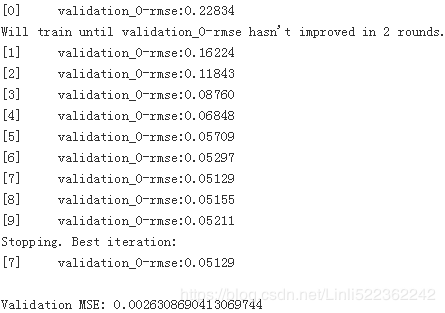
if xgboost is not None: #not shown in the book
    xgb_reg.fit( X_train, y_train,
                eval_set=[ (X_val, y_val)], early_stopping_rounds=2
               )
    y_pred = xgb_reg.predict( X_val )
    val_error = mean_squared_error( y_val, y_pred ) # Not shown
    print( "Validation MSE:", val_error)  #Not shown

%timeit xgboost.XGBRegressor().fit(X_train, y_train) if xgboost is not None else None

%timeit xgboost.XGBRegressor().fit(X_train, y_train) 

Stacking

     The last Ensemble method we will discuss in this chapter is called stacking (short for stacked generalization).
http://machine-learning.martinsewell.com/ensembles/stacking/Wolpert1992.pdf It is based on a simple idea: instead of using trivial不重要的 functions (such as hard voting) to aggregate the predictions of all predictors in an ensemble, why don't we train a model to perform this aggregation? Figure 7-12 shows such an ensemble performing a regression task on a new instance. Each of the bottom three predictors predicts a different value (3.1, 2.7, and 2.9), and then the final predictor (called a blender, or a meta learner) takes these predictions as inputs and makes the final prediction (3.0).

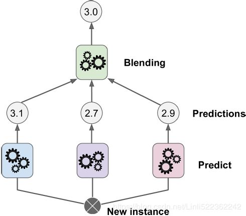
Figure 7-12. Aggregating predictions using a blending predictor
#######################

To train the (only one)blender, a common approach is to use a hold-out set.(Alternatively, it is possible to use out-of-fold predictions. In some contexts this is called stacking, while using a hold-out set is called blending混合. However, for many people these terms are synonymous) Let's see how it works. First, the training set is split in two subsets. The first subset(Subset 1) is used to train(this is a fit process) the predictors in the first layer (see Figure 7-13).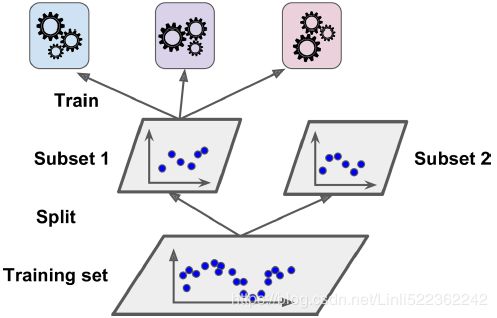
                               
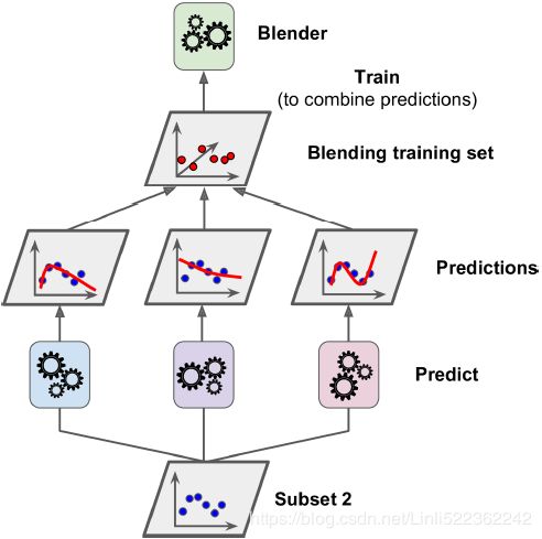
Figure 7-13. Training the first layer                                                     Figure 7-14. Training the blender in second layer
     Next, the first layer predictors are used to make predictions on the second (held-out) set((Subset 2)) (see Figure 7-14). This ensures that the predictions are“clean,” since the predictors never saw these instances during training.

     Now for each instance in the hold-out set(Subset 2) there are three predicted values(In other words, we use the held-out set and estimators of the first layer to make predictions). We can create a new training set using these predicted values as input features (which makes this new training set/Blending train set three-dimensional), and keeping the target values(Actual ys in held-out set or in (Subset 2)). The blender is trained on this blending training set, so it learns to predict the target value(Actual ys in held-out set or in (Subset 2)) given the first layer's predictions(we use an new instance and estimators of the first layer to make predictions).

the example is in the end of question 9 Stacking Ensemble
#######################

     It is actually possible to train several different blenders this way (e.g., one using Linear Regression, another using Random Forest Regression, and so on): we get a whole layer of blenders. The trick is to split the training set into three subsets: the first one is used to train the first layer(to train the predictors),

the second one is used to create the training set to train the second layer (using predictions made by the predictors of the first layer; In other words, we use the second one training set and estimators of the first layer to make predictions, then use the  new training set /Blending train set created by the predictions to train blenders), 

and the third one is used to create the training set to train the third layer ( we use the third one training set and estimators of the first layer to make predictions, then use these predictions and blenders (or estimators) in second layer to make predictions; finally use these predcitions to create a new training set again) ###(using the new training set or predictions made by the predictors or blenders of the second layer to train the predictor in 3rd layer)### . Once this is done, we can make a prediction for a new instance by going through each layer sequentially, as shown in Figure 7-15.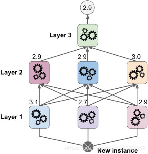

Figure 7-15. Predictions in a multilayer stacking ensemble

     Unfortunately, Scikit-Learn does not support stacking directly, but it is not too hard to roll out your own implementation (see the following exercises). Alternatively, you can use an open source implementation such as brew (available at https://github.com/viisar/brew).

Exercises

1. If you have trained five different models on the exact same training data, and they all achieve 95% precision, is there any chance that you can combine these models to get better results? If so, how? If not, why?

     If you have trained five different models and they all achieve 95% precision, you can try combining them into a voting ensemble, which will often give you even better results. It works better if the models are very different (e.g., an SVM classifier, a Decision Tree classifier, a Logistic Regression classifier, and so on). It is even better if they are trained on different training instances (that’s the whole point of bagging and pasting ensembles), but if not it will still work as long as the models are very different.

2. What is the difference between hard and soft voting classifiers?

Figure 7-2. Hard voting classifier predictions

     A hard voting classifier just counts the votes of each classifier in the ensemble and picks the class that gets the most votes. A soft voting classifier computes the average estimated class probability for each class and picks the class with the highest probability. This gives high-confidence votes more weight and often performs better, but it works only if every classifier is able to estimate class probabilities(e.g., for the SVM classifiers in Scikit-Learn you must set probability=True).

3. Is it possible to speed up training of a bagging ensemble by distributing it across multiple servers? What about pasting ensembles, boosting ensembles, random forests, or stacking ensembles?

           
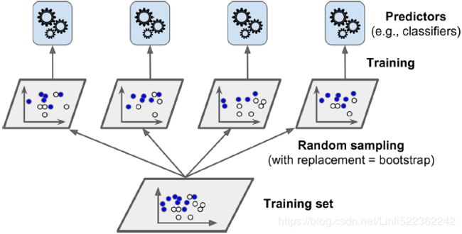
Figure 7-4. Pasting/bagging training set sampling and training         AdaBoost sequential training with instance weight updates

     It is quite possible to speed up training of a bagging ensemble by distributing it across multiple servers, since each predictor in the ensemble is independent of the others. The same goes for pasting(boostrap=False) ensembles and Random Forests(is an ensemble of Decision Trees, generally trained via the bagging method (or sometimes pasting) max_samples=1.0, #The number of samples to draw from X to train each base estimator. #max_samples * X.shape[0]), for the same reason. However, each predictor in a boosting ensemble is built based on the previous predictor, so training is necessarily sequential, and you will not gain anything by distributing training across multiple servers. Regarding stacking ensembles, all the predictors in a given layer are independent of each other, so they can be trained in parallel on multiple servers. However, the predictors in one layer can only be trained after the predictors in the previous layer have all been trained.
                           
Figure 7-13. Training the first layer                                                        Figure 7-14. Training the blender in second layer

4. What is the benefit of out-of-bag evaluation?

     With out-of-bag evaluation, each predictor in a bagging ensemble is evaluated using instances that it was not trained on (they were held out). This makes it possible to have a fairly unbiased evaluation of the ensemble without the need for an
additional validation set. Thus, you have more instances available for training, and your ensemble can perform slightly better.

5. What makes Extra-Trees(Extremely Randomized Trees ensemble) more random than regular Random Forests? How can this extra randomness help? Are Extra-Trees slower or faster than regular Random Forests?

     When you are growing a tree in a Random Forest, only a random subset of the features is considered for splitting at each node. This is true as well for Extra-Trees, but they go one step further: rather than searching for the best possible
thresholds, like regular Decision Trees do, they use random thresholds for each feature. This extra randomness acts like a form of regularization: if a Random Forest overfits the training data, Extra-Trees might perform better. Moreover, since Extra-Trees don’t search for the best possible thresholds, they are much faster to train than Random Forests. However, they are neither faster nor slower than Random Forests when making predictions.

6. If your AdaBoost ensemble underfits the training data, what hyperparameters should you tweak and how?

     If your AdaBoost ensemble underfits the training data, you can try increasing the number of estimators or reducing the regularization hyperparameters of the base estimator(svm_clf = SVC( kernel="rbf", C=0.05, gamma="scale", random_state=42 )). You may also try slightly increasing the learning rate.
Figure 7-8. Decision boundaries of consecutive predictors

Figure 7-8 shows the decision boundaries of five consecutive predictors on the moons dataset (in this example, each predictor is a highly regularized SVM classifier with an RBF kernel (This is just for illustrative purposes. SVMs are generally not good base predictors for AdaBoost, because they are slow and tend to be unstable with AdaBoost.)) The first classifier gets many instances wrong, so their weights get boosted. The second classifier therefore does a better job on these instances, and so on. The plot on the right represents the same sequence of predictors except that the learning rate is halved (i.e., the misclassified instance weights are boosted half as much at every iteration误分类实例权重每次迭代上升一半). As you can see, this sequential learning technique has some similarities with Gradient Descent, except that instead of tweaking a single predictor’s parameters to minimize a cost function, AdaBoost adds predictors to the ensemble, gradually making it better.

for example your base estimator 

svm_clf = SVC( kernel="rbf", C=0.05, gamma="scale", random_state=42 )#'rbf': Gaussian Radial Basis Function高斯辐射基函数

https://blog.csdn.net/Linli522362242/article/details/104280075

 minimize                                                                      

The width of the street is controlled by a hyperparameter ϵ(Epsilon , n: the index of instances)
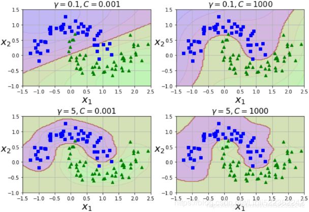
 The C parameter trades off correct classification of training examples against maximization of the decision function’s margin. For larger values of C, a smaller margin will be accepted if the decision function is better at classifying all training points correctly. A lower C will encourage a larger margin, therefore a simpler decision function, at the cost of training accuracy. In other words``C`` behaves as a regularization parameter(inversely)

where the parameter C > 0 controls the trade-off between the slack variable penalty and the margin. Because any point that is misclassified has ξn > 1, it follows that  is an upper bound on the number of misclassified points. The parameter C is therefore analogous相似的 to a regularization coefficient because it controls the trade-off between minimizing training errors and controlling model complexity. In the limit C → ∞, we will recover the earlier support vector machine for separable data
 

Gaussian RBF

Increasing gamma(γ) makes the bell-shape curve narrower (see the left plot of Figure 5-8 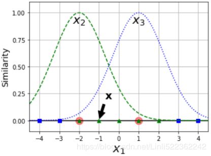 ), and as a result each instance’s range of influence is smaller: the decision boundary ends up being more irregular, wiggling扭动 around individual instances. Conversely, a small gamma(γ) value makes the bell-shaped curve wider, so instances have a larger range of influence, and the decision boundary ends up smoother. So γ acts like a regularization hyperparameter: if your model is overfitting, you should reduce it, and if it is underfitting, you should increase it (similar to the C hyperparameter).

7. If your Gradient Boosting ensemble overfits the training set, should you increase or decrease the learning rate?

     If your Gradient Boosting ensemble overfits the training set, you should try decreasing the learning rate. You could also use early stopping to find the right number of predictors (you probably have too many).

gbrt = GradientBoostingRegressor( max_depth=2, n_estimators=200, learning_rate=0.03, random_state=42 )
gbrt.fit( X,y )

                                                                 ###
gbrt_slow = GradientBoostingRegressor( max_depth=2, n_estimators=200, learning_rate=0.1, random_state=42 )
gbrt_slow.fit( X,y )

8. Load the MNIST data (introduced in https://blog.csdn.net/Linli522362242/article/details/103786116), and split it into a training set, a validation set, and a test set (e.g., use 40,000 instances for training, 10,000 for validation, and 10,000 for testing).

from sklearn.datasets import fetch_openml
mnist = fetch_openml("mnist_784")
mnist.keys()

 

mnist.data.shape

 

set(mnist.target)

 

from sklearn.model_selection import train_test_split

X_train_val, X_test, y_train_val, y_test = train_test_split(
    mnist.data, mnist.target, test_size=10000, random_state=42
)

X_train, X_val, y_train, y_val = train_test_split(
    X_train_val, y_train_val, test_size=10000, random_state=42
)

Then train various classifiers, such as a Random Forest classifier, an Extra-Trees classifier, and an SVM.

###################################
Why OvA or one-versus-the-rest?

https://blog.csdn.net/Linli522362242/article/details/103786116

Multiclass Classification
Whereas binary classifiers distinguish between two classes, multiclass classifiers (also called multinomial classifiers) can distinguish between more than two classes.

Some algorithms (such as Random Forest classifiers or naive Bayes classifiers) are capable of handling multiple classes directly. Others (such as Support Vector Machine classifiers or Linear classifiers) are strictly binary classifiers. However, there are various strategies that you can use to perform multiclass classification using multiple binary classifiers.

For example, one way to create a system that can classify the digit images into 10 classes (from 0 to 9) is to train 10 binary classifiers, one for each digit (a 0-detector, a 1-detector, a 2-detector, and so on). Then when you want to classify an image, you get the decision score from each classifier for that image and you select the class whose classifier outputs the highest score. This is called the one-versus-all (OvA) strategy (also called one-versus-the-rest).

Another strategy is to train a binary classifier for every pair of digits: one to distinguish 0s and 1s, another to distinguish 0s and 2s, another for 1s and 2s, and so on. This is called the one-versus-one (OvO) strategy. If there are N classes, you need to train N × (N – 1) / 2 classifiers. For the MNIST problem, this means training 45 binary classifiers! When you want to classify an image, you have to run the image through all 45 classifiers and see which class wins the most duels竞争. The main advantage of OvO is that each classifier only needs to be trained on the part of the training set for the two classes that it must distinguish.
###################################
Why linear SVM?

https://blog.csdn.net/Linli522362242/article/details/104403372
5. Should you use the primal or the dual form of the SVM problem to train a model on a training set with millions of instances and hundreds of features?
     This question applies only to linear SVMs since kernelized can only use the dual form. The computational complexity of the primal form of the SVM problem is proportional to the number of training instances m, while the computational complexity of the dual form is proportional to a number between  and . So if there are millions of instances(here, this exercise just has 70000 instances), you should definitely use the primal form, because the dual form will be much too slow.

Equation 5-13. Linear SVM classifier cost function
 
     The first sum in the cost function will push the model to have a small weight vector w, leading to a larger margin. The second sum computes the total of all margin violations. An instance’s margin violation is equal to 0 if it is located off the street and on the correct side, or else it is proportional成比例的 to the distance to the correct side of the street. Minimizing this term ensures that the model makes the margin violations as small and as few as possible.
###################################
Why Extra-Trees?

A forest of such extremely random trees is simply called an Extremely Randomized Trees ensemble 极端随机树(or Extra-Trees for short). Once again, this trades more bias for a lower variance. It also makes Extra-Trees much faster to train than regular Random Forests since finding the best possible threshold for each feature at every node is one of the most time-consuming tasks of growing a tree.

5. What makes Extra-Trees(Extremely Randomized Trees ensemble) more random than regular Random Forests? How can this extra randomness help? Are Extra-Trees slower or faster than regular Random Forests?

     When you are growing a tree in a Random Forest, only a random subset of the features is considered for splitting at each node. This is true as well for Extra-Trees, but they go one step further: rather than searching for the best possible thresholds, like regular Decision Trees do, they use random thresholds for each feature. This extra randomness acts like a form of regularization: if a Random Forest overfits the training data, Extra-Trees might perform better. Moreover, since Extra-Trees don’t search for the best possible thresholds, they are much faster to train than Random Forests. However, they are neither faster nor slower than Random Forests when making predictions.

###################################
Then train various classifiers, such as a Random Forest classifier, an Extra-Trees classifier, and an SVM.

from sklearn.ensemble import RandomForestClassifier, ExtraTreesClassifier
from sklearn.svm import LinearSVC
from sklearn.neural_network import MLPClassifier

random_forest_clf = RandomForestClassifier(n_estimators=10, random_state=42)
extra_trees_clf = ExtraTreesClassifier(n_estimators=10, random_state=42)
svm_clf = LinearSVC(random_state=42)
mlp_clf = MLPClassifier(random_state=42)


estimators = [ random_forest_clf, extra_trees_clf, svm_clf, mlp_clf ]
for estimator in estimators:
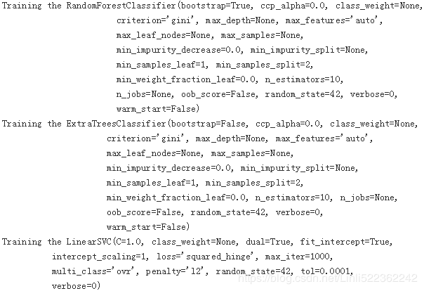
    print( "Training the", estimator)
    estimator.fit(X_train, y_train)

 

[estimator.score(X_val, y_val) for estimator in estimators]

 ####################

from sklearn.ensemble import RandomForestClassifier, ExtraTreesClassifier
from sklearn.svm import LinearSVC
from sklearn.neural_network import MLPClassifier
                                          #################
random_forest_clf = RandomForestClassifier(n_estimators=100, random_state=42)
extra_trees_clf = ExtraTreesClassifier(n_estimators=100, random_state=42)
svm_clf = LinearSVC(random_state=42)
mlp_clf = MLPClassifier(random_state=42)

estimators = [ random_forest_clf, extra_trees_clf, svm_clf, mlp_clf ]
for estimator in estimators:
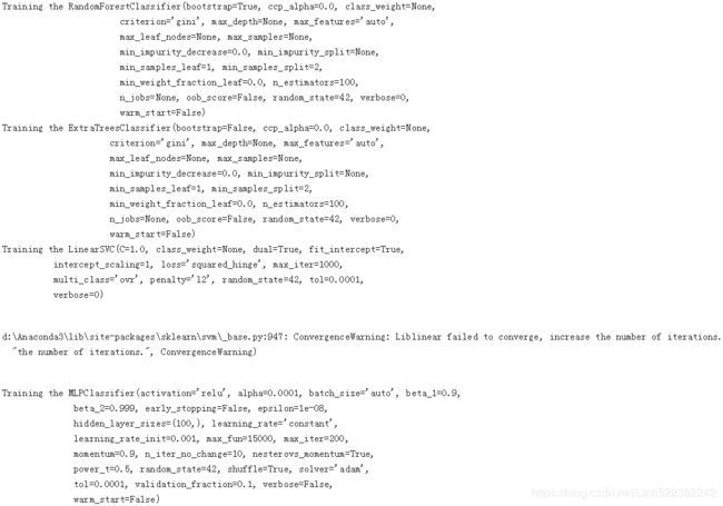
    print( "Training the", estimator)
    estimator.fit(X_train, y_train)

[estimator.score(X_val, y_val) for estimator in estimators]

 ###########
Both RandomForestClassifier and ExtraTreesClassifier with n_estimators=100 are better than if they just have 10 estimators. ( VS )

The linear SVM is far outperformed by the other classifiers. However, let's keep it for now since it may improve the voting classifier's performance.

A very simple way to create an even better classifier is to aggregate the predictions of each classifier and predict the class that gets the most votes. This majority-vote classifier is called a hard voting classifier (see Figure 7-2).

Figure 7-2. Hard voting classifier predictions

Next, try to combine them into an ensemble that outperforms them all on the validation set, using a soft or hard voting classifier. Once you have found one, try it on the test set. How much better does it perform compared to the individual classifiers?

from sklearn.ensemble import VotingClassifier

named_estimators =[
    ("random_forest_clf", random_forest_clf),
    ("extra_trees_clf", extra_trees_clf),
    ("svm_clf", svm_clf),
    ("mpl_clf", mlp_clf),
]

voting_clf = VotingClassifier(named_estimators)
voting_clf.fit(X_train,y_train)

voting_clf.score(X_val, y_val)

[estimator.score(X_train, y_train) for estimator in voting_clf.estimators_]

note: some people may get the result of which is same with [estimator.score(X_val, y_val) for estimator in estimators] before combining

Let's remove the SVM to see if performance improves. It is possible to remove an estimator by setting it to None using set_params() like this:

voting_clf.set_params(svm_clf=None)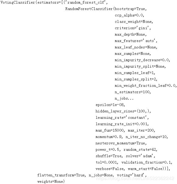

This updated the list of estimators:

voting_clf.estimators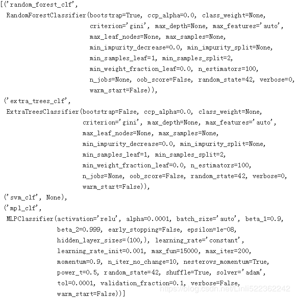

However, it did not update the list of trained estimators:

voting_clf.estimators_

So we can either fit the VotingClassifier again, or just remove the SVM from the list of trained estimators: 

del voting_clf.estimators_[2]

Now let's evaluate the VotingClassifier again: 

voting_clf.score(X_val, y_val)

A bit better! The SVM was hurting performance. Now let's try using a soft voting classifier. We do not actually need to retrain the classifier, we can just set voting to "soft" and ensure that all classifiers can estimate class probabilities:

voting_clf.voting = "soft"
voting_clf.score(X_val, y_val)

Nope, hard voting wins in this case.

voting_clf.voting = "hard"
voting_clf.score(X_test, y_test)

[estimator.score(X_test, y_test) for estimator in estimators if estimator is not svm_clf]

The voting classifier only very slightly reduced the error rate of the best model (0.9691) in this case.
                         
Figure 7-13. Training the first layer                                               Figure 7-14. Training the blender in second layer

estimators

 

9. Stacking Ensemble

9. Run the individual classifiers from the previous exercise to make predictions on the validation set, and create a new training set with the resulting predictions: each training instance is a vector containing the set of predictions from all your classifiers for an image, and the target is the image's class.

Train a classifier on this new training set.

#to get predictions by using previous(first layer's) estimators and second layer's training set(X_val)

X_val_predictions = np.empty( (len(X_val), len(estimators) ), dtype=np.float32 )

for index, estimator in enumerate( estimators ):
    X_val_predictions[:,index] = estimator.predict(X_val)

X_val_predictions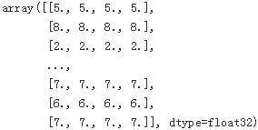

 
# use previous predictions to create a blending train set then to train blender

rnd_forest_blender = RandomForestClassifier(n_estimators=200, oob_score=True, random_state=42)
rnd_forest_blender.fit(X_val_predictions, y_val)

 

rnd_forest_blender.oob_score_

 
You could fine-tune this blender or try other types of blenders (e.g., an MLPClassifier), then select the best one using cross-validation, as always.

Congratulations, you have just trained a blender, and together with the classifiers they form a stacking ensemble! Now let’s evaluate the ensemble on the test set. For each image in the test set, make predictions with all your classifiers, then feed the predictions to the blender to get the ensemble’s predictions. How does it compare to the voting classifier you trained earlier?

#to get an new predictions by using first layer's  estimators and the test set

X_test_predictions = np.empty( (len(X_test), len(estimators)), dtype=np.float32 )

for index, estimator in enumerate(estimators):
    X_test_predictions[:, index] = estimator.predict(X_test)

# to make final predictions by using an new training dataset( from previous predctions) and blender in second layer 

y_pred = rnd_forest_blender.predict( X_test_predictions )

from sklearn.metrics import accuracy_score

accuracy_score(y_test, y_pred)

 

This stacking ensemble does not perform as well as the voting classifier we trained earlier, it's not quite as good as the best individual classifier.