图像边缘检测的Sobel和Laplace算子和图像最近邻插值和双线性插值算法的Python实现（附完整代码）

1.概述

计算机视觉课程要求实现一下图像边缘检测算法，但并没有明确要求实现哪种具体的算法，在网上看了相关图像边缘检测算子，都有非常具体的介绍，也有实现代码或者Python集成库里的代码，有的算子比较简单，很容易理解，例如Sobel、Laplace等，Sobel还有一系列延伸的算子，很相似，这些都还是比较简单的，还有一些稍微复杂点的算子，例如Canny，具体关于这些算法原理的介绍推荐去看深入学习OpenCV中几种图像边缘检测算子这篇文章，写的非常棒。看了一些博主写的代码，写的非常好，但是跟我想象中所要求的还是有一些出入，所以我在这个代码的基础上进行了一些修改。本次作业我选择了实现Sobel和Laplace两个比较简单的算法，这里作个记录。

2.Sobel和Laplace简单介绍和实现

2.1 Sobel算子

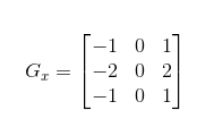
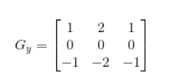
Sobel算子包括横向和纵向两种模板，把横向模板记为$Gx$，把纵向模板记为$Gy$，其中：

在计算时，首先需要将图像转成灰度图，直接用下面的方法即可，参数$0$代表读取灰度图。

gray_saber = cv2.imread("C:/Users/ALIENWARE/Pictures/Camera Roll/mcqueen.jpg",0)

然后只需要将上述模板看成一个“元素矩阵”或者“基本矩阵”，然后依次与灰度图中每个相同大小的矩阵进行相乘（当然，图像中每个矩阵中的值都代表图中的灰度值），然后将每个矩阵与“基本矩阵”相乘之后所有元素求和，即：
$$\begin{gathered} G{x}^{\prime }=sum(Gx\ast A_i) \\ G{y}^{\prime }=sum(Gy\ast A_i) \end{gathered}$$其中$A$为灰度图矩阵，$A_i$即代表灰度图矩阵中每个大小为$3\times 3$的矩阵，$sum()$就代表将矩阵中所有元素求和操作。

def SobelOperator(roi, operator_type):
    if operator_type == "horizontal":
        sobel_operator = np.array([[-1, -2, -1], [0, 0, 0], [1, 2, 1]]) #横向模板
    elif operator_type == "vertical":
        sobel_operator = np.array([[-1, 0, 1], [-2, 0, 2], [-1, 0, 1]]) #纵向模板
    else:
        raise ("type Error")
    result = np.abs(np.sum(roi * sobel_operator))
    return result

这样计算之后，再取这两个模板结果的几何平均值作为每个坐标位置的新的灰度值（其实这样必然会造成图片上某些点没有被处理，但是几乎没有什么影响），即：
$$G=\sqrt{{G{x}^{\prime }}^2+{G{y}^{\prime }}^2}$$
实现代码如下：

def SobelAlogrithm(image):
    new_image1 = np.zeros(image.shape)
    new_image2 = np.zeros(image.shape)
    for i in range(1, image.shape[0] - 1):
        for j in range(1, image.shape[1] - 1):
            new_image1[i - 1, j - 1] = SobelOperator(image[i - 1:i + 2, j - 1:j + 2], 'horizontal')
            new_image2[i - 1, j - 1] = SobelOperator(image[i - 1:i + 2, j - 1:j + 2], 'vertical')
    new_image1 = np.sqrt(new_image1*new_image1+new_image2*new_image2)
    new_image1 = 255 - new_image1*(255 / np.max(new_image1))        #将图片像素值取反
    return new_image1.astype(np.uint8)

2.2 LapLace算子

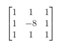
Laplace算子的操作过程与Sobel算子基本一样，但是原理肯定大不相同。Laplace算子具有4邻域模板和8邻域模板，与Sobel算子不同的是，Sobel算子在计算最终图像的灰度值时，需要同时利用到横向模板和纵向模板计算的结果，而Laplace算子的两个模板只是多了一种选择，可以根据不同情况选择使用哪种模板进行操作。4邻域模板和8邻域模板分别为：

同样的，把模板看做为“元素矩阵”或“基本矩阵”与灰度图矩阵相乘，并将相乘得到的矩阵中所有元素求和，作为图像对应坐标位置的灰度值。（这里以4邻域模板$G_4$作为例子）
$$G=sum(G_4\ast A_i)$$代码如下：

def LaplaceOperator(roi, operator_type):
    if operator_type == "fourfields":
        laplace_operator = np.array([[0, 1, 0], [1, -4, 1], [0, 1, 0]])
    elif operator_type == "eightfields":
        laplace_operator = np.array([[1, 1, 1], [1, -8, 1], [1, 1, 1]])
    else:
        raise ("type Error")
    result = np.abs(np.sum(roi * laplace_operator))
    return result

3.实验结果与完整代码

3.1 实验结果

首先放张原图（太白山游客照）

读取到的灰度图为

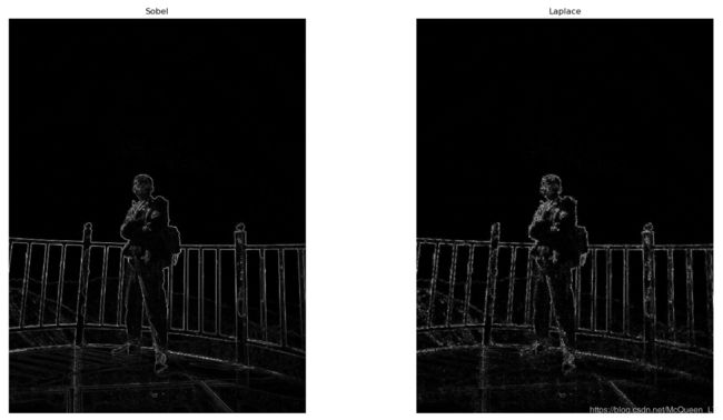
最后用Sobel和Laplace方法得到的边缘检测结果如下

3.2 完整代码

接下来就是完整代码了！！！

import cv2
import matplotlib.pyplot as plt
import numpy as np

def SobelOperator(roi, operator_type):
    if operator_type == "horizontal":
        sobel_operator = np.array([[-1, -2, -1], [0, 0, 0], [1, 2, 1]])
    elif operator_type == "vertical":
        sobel_operator = np.array([[-1, 0, 1], [-2, 0, 2], [-1, 0, 1]])
    else:
        raise ("type Error")
    result = np.abs(np.sum(roi * sobel_operator))
    return result

def SobelAlogrithm(image):
    new_image1 = np.zeros(image.shape)
    new_image2 = np.zeros(image.shape)
    for i in range(1, image.shape[0] - 1):
        for j in range(1, image.shape[1] - 1):
            new_image1[i - 1, j - 1] = SobelOperator(image[i - 1:i + 2, j - 1:j + 2], 'horizontal')
            new_image2[i - 1, j - 1] = SobelOperator(image[i - 1:i + 2, j - 1:j + 2], 'vertical')
    new_image1 = np.sqrt(new_image1*new_image1+new_image2*new_image2)
    new_image1 = 255 - new_image1*(255 / np.max(new_image1))
    return new_image1.astype(np.uint8)

def LaplaceOperator(roi, operator_type):
    if operator_type == "fourfields":
        laplace_operator = np.array([[0, 1, 0], [1, -4, 1], [0, 1, 0]])
    elif operator_type == "eightfields":
        laplace_operator = np.array([[1, 1, 1], [1, -8, 1], [1, 1, 1]])
    else:
        raise ("type Error")
    result = np.abs(np.sum(roi * laplace_operator))
    return result


def LaplaceAlogrithm(image, operator_type):
    new_image = np.zeros(image.shape)
    image = cv2.copyMakeBorder(image, 1, 1, 1, 1, cv2.BORDER_DEFAULT)
    for i in range(1, image.shape[0] - 1):
        for j in range(1, image.shape[1] - 1):
            new_image[i - 1, j - 1] = LaplaceOperator(image[i - 1:i + 2, j - 1:j + 2], operator_type)
    new_image = 255-new_image * (255 / np.max(image))
    return new_image.astype(np.uint8)

gray_saber = cv2.imread("C:/Users/ALIENWARE/Pictures/Camera Roll/mcqueen.jpg",0)

plt.subplot(121)
plt.title("Sobel")
plt.imshow(SobelAlogrithm(gray_saber),cmap="binary")
plt.axis("off")
plt.subplot(122)
plt.title("Laplace")
plt.imshow(LaplaceAlogrithm(gray_saber, "fourfields"), cmap="binary")
plt.axis("off")
plt.show()

最后，再次感谢深入学习OpenCV中几种图像边缘检测算子这边文章！！！

补充一个图像最近邻插值和双线性插值算法的代码（就是把代码存在这里，等有时间了在好好整理一下）

import cv2
import numpy as np
import matplotlib.pyplot as plt

def nearestInterpolation(originImg, scale):
    newImgRows = round(originImg.shape[0]*scale)
    newImgCols = round(originImg.shape[1]*scale)

    newImg = np.zeros(shape= [newImgRows,newImgCols,3],dtype=np.uint8) #3通道图像
    for i in range(newImg.shape[0]):
        for j in range(newImg.shape[1]):
            row_int = round(i/scale)
            col_int = round(j/scale)
            if row_int == originImg.shape[0] or col_int == originImg.shape[1]:
                row_int -= 1
                col_int -= 1
            newImg[i][j] = originImg[row_int][col_int]
    return newImg

def bilinearInterpolation(originImg, scale):
    newImgRows = round(originImg.shape[0]*scale)
    newImgCols = round(originImg.shape[1]*scale)

    newImg = np.zeros(shape=[newImgRows,newImgCols,3],dtype=np.uint8)
    for i in range(newImg.shape[0]):
        for j in range(newImg.shape[1]):
            row = i/scale
            col = j/scale
            row_int = int(row)
            col_int = int(col)
            u = row-row_int
            v = col-col_int
            if row_int == originImg.shape[0]-1 or col_int == originImg.shape[1]-1:
                row_int -= 1
                col_int -= 1

            newImg[i][j] = (1-u)*(1-v)*originImg[row_int][col_int]+(1-u)*v*originImg[row_int][col_int+1]+\
                     + u * (1 - v) * originImg[row_int + 1][col_int] + u * v * originImg[row_int + 1][col_int + 1]

    return newImg


if __name__ == '__main__':
    img = cv2.imread("C:/Users/ALIENWARE/Pictures/Camera Roll/mcqueen.jpg",1)

    method = int(input('choose a method(1/nearest 2/bilinear): '))
    scale = float(input('input a scale you want: '))
    if method == 1:
        newImg = nearestInterpolation(img,scale)
    if method == 2:
        newImg = bilinearInterpolation(img,scale)

    print("new img's shape is: ",newImg.shape)

    newImg = cv2.cvtColor(newImg, cv2.COLOR_RGB2BGR)
    plt.title('newImg')
    plt.imshow(newImg)
    plt.show()

    img = cv2.cvtColor(img,cv2.COLOR_RGB2BGR)
    plt.title('img')
    plt.imshow(img)
    plt.show()