Chapter 6 决策树

OReilly.Hands-On Machine Learning with Scikit-Learn and TensorFlow读书笔记

Chapter 6 Decision Trees

Like SVMs, Decision Trees are versatile ML algorithms that can perform both classification and regression tasks, and even multioutput tasks.

Decision Trees are also fundamental components of Random Forest, which are among the most powerful ML algorithms.

6.1 Training and Visualizing a Decision Tree

Training a $\text{DecisionTreeClassifier}$ on the iris dataset.

from sklearn.datasets import load_iris
from sklearn.tree import DecisionTreeClassifier
iris=load_iris()

#receive different results, why?
#X=iris['data'][:,2:] #petal length and width
#y=iris['target']

X=iris.data[:,2:]
y=iris.target

tree_clf=DecisionTreeClassifier(max_depth=2)
tree_clf.fit(X,y)

In your working directory, manually create directories of the following structure: ./images/decision_trees

You can visualize the trained decision tree by using the $\text{export\_graphviz()}$ method to output a graph definition file called iris_tree.dot.

from sklearn.tree import export_graphviz
import os
# Where to save the figures
PROJECT_ROOT_DIR = "."
CHAPTER_ID = "decision_trees"

def image_path(fig_id):
    return os.path.join(PROJECT_ROOT_DIR, "images", CHAPTER_ID, fig_id)

export_graphviz(
    tree_clf,
    out_file=image_path("iris_tree.dot"),
    feature_names=iris.feature_names[2:],
    class_names=iris.target_names,
    rounded=True,
    filled=True
)

Then you can convert this .dot file to a variety formats such as PDF or PNG using the dot command-line tool from the graphviz package.

$dot -Tpng iris_tree.dot -o iris_tree.png

6.2 Making Predictions

One of the many qualities of Decision Trees is that they require very little data preparation. In particular, they don’t require feature scaling or centering at all.

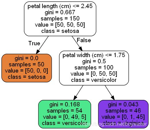
A node’s $\text{samples}$ attribute counts how many training instances it applies to.

A node’s $\text{value}$ attribute tells you how many training instances of each class this node contains.

A node’s $\text{gini}$ attribute measures its impurity: a node is “pure” ($\text{gini=0}$) if all training instances it applies to belong to the same class.

Equation 6-1. Gini impurity
$$G_i=1-\sum _{k=1}^n{p}_{i,k}^2$$

• $p_{i,k}$ is the ratio of class $k$ instances among the training instances in the $i$-th node.

For example, the depth-2 left node has a $\text{gini}$ score equal to $1–(0/54{)}^2–(49/54{)}^2–(5/54{)}^2\approx 0.168$.

Scikit-Learn uses the CART algorithm, which produces only binary trees. Other algorithms such as ID3 can produce Decision Trees with nodes that have more than two children.

Model Interpretation: White Box Versus Black Box

White Box Models are fairly intuitive and their decisions are easy to interpret, such as Decision Trees.

Black box models are usually hard to explain in simple terms why the predictions were made, such as Random Forest and Neural Networks.

6.3 Estimating Class Probabilities

tree_clf.predict_proba([[5,1.5]])
#array([[0.        , 0.90740741, 0.09259259]])
tree_clf.predict([[5,1.5]])#array([1])

6.4 The CART Training Algorithm

Scikit-Learn use CART (Classification And Regression Tree) algorithm to train Decision Trees (this process is also called “growing” trees). The idea is: the algorithm first splits the training set in two subsets using a single feature $k$ and a threshold $t_k$ (e.g., “petal length $\le$ 2.45 cm”).

How does it choose $k$ and $t_k$?

It searches for the pair $(k,t_k)$ that produces the purest subsets (weighted by their size). The cost function that the algorithm tries to minimize is given by Equation 6-2.

Equation 6-2. CART cost function for classification
$$\begin{gathered} J(k,t_k)=\frac{m_{\text{left}}}{m}{G}_{\text{left}}+\frac{m_{\text{right}}}{m}{G}_{\text{right}} \\ \text{where }\{\begin{array}{l}{G}_{\text{left/right}}\text{ measures the impurity of the left/right subsets,}\\ m_{\text{left/right}}\text{ is the number of instances in the left/right subsets,}\end{array} \end{gathered}$$
Termination conditions: It stops recursing once it reaches the maximum depth (defined by the $\text{max\_depth}$ hyperparameter), or if it cannot find a split that will reduce impurity. A few other hyperparameters control additional stopping conditions ($\text{min\_samples\_split}$, $\text{min\_samples\_leaf}$, $\text{min\_weight\_fraction\_leaf}$, and $\text{max\_leaf\_nodes}$).

The CART algorithm is a greedy algorithm: it greedily searches for an optimum split at the top level, then repeat the process at each level. It does not check whether or not the split will lead to the lowest possible impurity several levels down. A greedy algorithm often produces a reasonably good solution, but it is not guaranteed to be the optimal solution.

Finding the optimal tree is known to be an NP-Complete problem.

6.5 Computational Complexity

Traversing the Decision Tree requires going through roughly $O({\log }_2(m))$ nodes. Since each node requires checking the value of one feature, the overall prediction complexity is just $O({\log }_2(m))$, independent of the number of features.

However, the training algorithm compares all features (or less if $\text{max\_features}$ is set) on all samples at each node. This results in a training complexity of $O(n\times m{\log }_2(m))$.

For small training sets (less than a few thousand instances), Scikit-Learn can speed up
training by presorting the data (set $\text{presort=True}$), but this slows down training considerably for larger training sets.

6.6 Gini Impurity or Entropy?

Gini impurity measure is the default measurement, but you can use entropy impurity measure instead by setting the $\text{criterion}$ hyperparameter to “$\text{entropy}$”.

Equation 6-3. Entropy
$$H_i=-\underset{P_{i,k}̸=0}{\sum _{k=1}^n}{P}_{i,k}\log P_{i,k}$$
So should you use Gini impurity or entropy? The truth is, most of the time it does not
make a big difference: they lead to similar trees. Gini impurity is slightly faster to compute, so it is a good default. However, when they differ, Gini impurity tends to isolate the most frequent class in its own branch of the tree, while entropy tends to produce slightly more balanced trees.

6.7 Regularization Hyperparameters

Decision Trees make very few assumptions about the training data (as opposed to lin‐
ear models, which obviously assume that the data is linear, for example).

nonparametric model: the number of parameters is not determined prior to training, so the model structure is free to stick closely to the data.

parametric model: has a predetermined number of parameters, so its degree of freedom is limited, reducing the risk of overfitting (but increasing the risk of underfitting).

Regularization:

• $\text{max\_depth}$
• $\text{min\_samples\_split}$ (the minimum number of samples a node must have before it can be split)
• $\text{min\_samples\_leaf}$ (the minimum number of samples a leaf node must have)
• $\text{min\_weight\_fraction\_leaf}$ (same as $\text{min\_samples\_leaf}$ but expressed as a fraction of the total number of weighted instances)
• $\text{max\_leaf\_nodes}$ (maximum number of leaf nodes)
• $\text{max\_features}$ (maximum number of features that are evaluated for splitting at each node).

Increasing $\text{min\_*}$ hyperparameters or reducing $\text{max\_*}$ hyperparameters will regularize the
model (i.e., not making the model too complex).

Other algorithms work by first training the Decision Tree without restrictions, then pruning (deleting) unnecessary nodes. The necessity of pruning a node is evaluates by standard statistical tests, such as the ${\chi }^2$ test.

6.8 Regression

# Quadratic training set + noise
import numpy as np
np.random.seed(42)
m = 200
X = np.random.rand(m, 1)
y = 4 * (X - 0.5) ** 2
y = y + np.random.randn(m, 1) / 10
from sklearn.tree import DecisionTreeRegressor
tree_reg=DecisionTreeRegressor(max_depth=2)
tree_reg.fit(X,y)

export_graphviz(
    tree_reg,
    out_file=image_path("reg_tree.dot"),
    feature_names=['x1'],
    rounded=True,
    filled=True
)

$dot -Tpng reg_tree.dot -o reg_tree.png

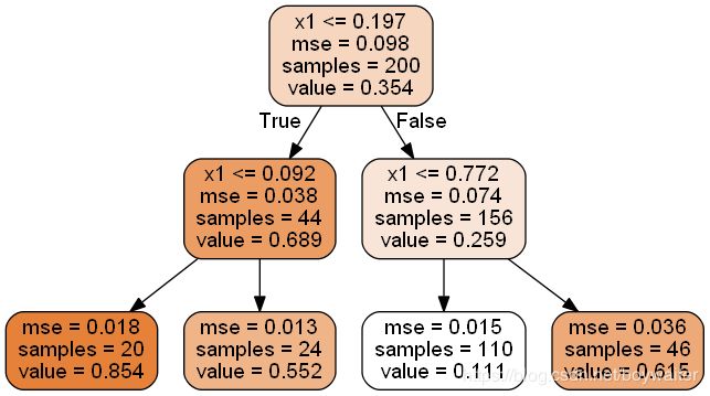
The main difference is that, given a $x_1$ value, instead of predicting a class in each node, it predicts a value. For example, the prediction of a new instance with $x_1=0.6$, the algorithm traverses the decision tree above, reaches the second to right leaf node, and obtain the value 0.111 finally. This prediction is simply the average target value of the 110 training instances associated to this leaf node. This prediction results in a mse (Mean Squared Error) equal to 0.015 over these 110 instances.

The CART algorithm works mostly the same way as earlier, except that instead of try‐
ing to split the training set in a way that minimizes impurity, it now tries to split the
training set in a way that minimizes the MSE.

Equation 6-4. CART cost function for regression
$$J(k,t_k)=\frac{m_{\text{left}}}{m}{\text{MSE}}_{\text{left}}+\frac{m_{\text{right}}}{m}{\text{MSE}}_{\text{right}}\text{where }\{\begin{array}{l}{\text{MSE}}_{\text{node}}={\sum }_{i\in \text{node}}{\left({\hat{y}}_{\text{node}}-y^{(i)}\right)}^2\\ {\hat{y}}_{\text{node}}=\frac{1}{m_{\text{node}}}{\sum }_{i\in \text{node}}{y}^{(i)}\end{array}$$

6.9 Instability

limitations:

• orthogonal decision boundaries (all splits are perpendicular to an axis), which makes them sensitive to training set rotation. One way to limit this is PCA.
• very sensitive to small variations in the training data