paper reading：Part-based Graph Convolutional Network for Action Recognition

paper reading：Part-based Graph Convolutional Network for Action Recognition

graph 与 skeleton：

Human skeleton is intuitively represented as a sparse graph with joints as nodes and natural connections between them as edges.

• nodes：joints
• edges：natural connections between joints

---

传统的 action recognition from S-videos：

• the whole skeleton is treated as a single graph
• 使用 3D coordinate

---

本文模型使用的两种信息：

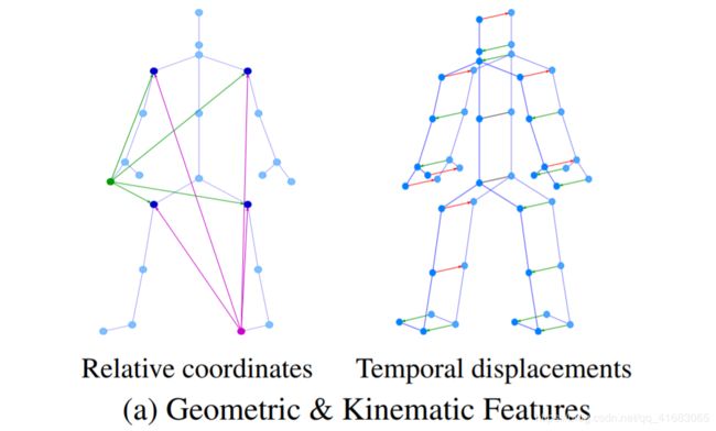
• Geometric features：such as relative joint coordinates
• motion features：such as temporal displacements

---

本文主要贡献：

• Formulation of a general part-based graph convolutional network (PB-GCN) .

• Use of geometric and motion features in place of 3D joint locations at each vertex.

  即，几何信息（relative joint coordinates）和运动信息（temporal displacements）的使用

• Exceeding the state-of-the-art on challenging benchmark datasets NTURGB+D and HDM05.

---

单图（无划分）的卷积公式：

k-th neighborhood

$$Y(v_i)=\sum _{v_j\in N_k(v_i)}W(L(v_j))X(v_j)$$

• $W(\cdot )$： a filter weight vector of size of $L$ indexed by the label assigned to neighbor $v_j$ in the $k$-neighborhood $N_k(v_i)$
• $X(v_j)$：the input feature at $v_j$
• $Y(v_j)$ ：convolved output feature at root vertex $v_i$

---

1-th neighborhood

将邻域$N_k(v_i)$换一种表示形式（用邻接矩阵$A$表示），且将邻域数从$k$降为1，则得到下面的式子
$$Y(v_i)=\sum _j{A}^{norm}(i,j)W(L(v_j))X(v_j)$$

• $D(i,i)={\sum }_j(i,j)$；$A^{norm}=D^{-1/2}A{D}^{-1/2}$

---

Part-based Graph

In general, a part-based graph can be constructed as a combination of subgraphs where each subgraph has certain properties that define it.

图的划分的定义：

We consider scenarios in which the partitions can share vertices or have edges connecting them.

即，一个图被划分为不同的子图，不同的子图会共享顶点或共享边。
$$G=\bigcup _{p\in \{1,...,n\}}{P}_p|P_p=(V_p,{\epsilon }_p)$$

• $P_p$ is the partition (or subgraph) $p$ of the graph $G$

two parts (b)：

• Axial skeleton
• Appendicular skeleton

four parts (c ) （推荐）：

• head
• hands
• torso
• legs

We consider left and right parts of hands and legs together in order to be agnostic to laterality [31] (handedness / footedness) of the human when performing an action.

即，排除侧向性的干扰（左手招手和右手招手都是招手）。

six part (d) ：

we divide the upper and lower components of appendicular skeleton into left and right (shown in Figure 1(d)), resulting in six parts

子图的连接：

图的连接有两种方式：点连接 & 边连接。此处采用的是点连接。

To cover all natural connections between joints in skeleton graph, we include an overlap of at least one joint between two adjacent parts.

即，每个子图之间有至少有一个公用的node。

---

Part-based Graph Convolutions

不同于上述提到的单图的卷积公式（Eq.2） ，划分为子图后，graph有新的卷积公式。

同时，有几个概念需要重新定义。

邻域：

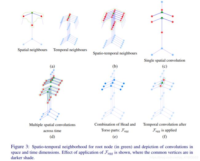
• 空间邻域（Spatial neighbor）：单个 frame 下（特定时间）一阶邻域（Figure 3(a)）。
• 时间邻域（Temporal neighbor）：单个 node 的 不同的时间的位置（Figure 3(a)）。
• 时空邻域（Spatial-temporal neighbor）：时空邻域的并集（Figure 3(b)）。

---

卷积：

graph convolutions over a part identifies the properties of that subgraph and an aggregation across subgraphs learns the relations between them.

For a part-based graph, convolutions for each part are performed separately and the results are combined using an aggregation function $F_{agg}$

即，先通过子图内卷积（一阶邻域），再通过聚合函数$F_{agg}$计算各子图的联系。

公式表达如下：

子图卷积：

$$Y_p(v_i)=\sum _{v_j\in N_{kp}(v_i)}{W}_p(L_p(v_j))X_p(v_j),p\in 1,...,n$$

• $W_p$ can be shared across parts or kept separate, while the neighbors of $v_i$ only in that part ($N_{kp}(v_i)$) are considered

子图卷积结果聚合：

边共享形式：
$$Y(v_i)=F_{agg}(Y_{p1}(v_i),Y_{p2}(v_j))|(v_i,v_j)\in \epsilon (p1,p2),(p1,p2)\in \{1,...,n\}\times \{1,...,n\}$$
顶点共享形式：
$$Y(v_i)=F_{agg}(Y_{p1}(v_i),Y_{p2}(v_i))|(p1,p2)\in \{1,...,n\}\times \{1,...,n\}$$

---

Spatio-temporal Part-based Graph Convolutions

卷积的步骤

The S-videos are represented as spatio-temporal graphs.

即，S-video 的本质是 spatio-temporal graphs.

we spatially convolve each partition independently for each frame, aggregate them at each frame and perform temporal convolution on the temporal dimension of the aggregated graph.

即大致分为两步，细致可分为3步：

• Spatial convolution（空间卷积）：
  • 子图卷积：spatially convolve each partition independently for each frame
  • 子图卷积结果聚合：aggregate result of partition convolution at each frame
• Temporal convolution（时间卷积）：
  • 对聚合结果进行时间卷积：temporal convolution on the temporal dimension of the aggregated graph。

---

邻域的划分

For each vertex, we use 1-neighborhood ($k$ = 1) for spatial dimension ($N_1$) as the skeleton graph is not very large and a $\tau$-neighborhood ($k$ = $\tau$) for the temporal dimension ($N_{\tau }$ ), $N_{\tau }$ is not part-specific.

空间邻域和时间邻域的划分，由下式表示：
$$N_{1p}(v_i)=\{v_j|d(v_i,v_j)\le 1,v_i,v_j\in V_p\}$$

$$N_{\tau }(v_{i{t}_a})=\{v_{i{t}_b}|d(v_{i{t}_a},v_{i{t}_b})\le |\frac{\tau }{2}|\}$$

---

标签的给定

For ordering vertices in the receptive fields (or neighborhoods), we use a single label spatially ($L_S:V\to \{0\})$ to weigh vertices in $N_{1p}$ of each vertex equally and $\tau$ labels temporally ($L_T:V\to \{0,...,\tau -1\}$) to weigh vertices across frames in $N_{\tau }$ differently.

即，对于 root 节点，空间邻域内 label 相同（为0），时间邻域内 label 不同。

公式表达如下：
$$L_S(v_{jt})=\{0|v_{jt}\in N_{1p}(v_{it})\}$$

$$L_T(v_{i{t}_b})=\{((t_b-t_a)+|\frac{\tau }{2}|)|v_{i{t}_b}\in N_{\tau }(v_{i{t}_a})\}$$

---

卷积的全部公式！！！

子图的空间卷积

$$Z_p(v_{jt})=W_p(L_S(v_{jt}))X_p(v_{jt})$$

• $W_p\in {\mathbb{R}}^{C{}^{\prime }\times C\times 1\times 1}$：part-specific channel transform kernel (pointwise operation)
• $L_S$ for each part is same but $N_{1p}$ is part-specific
• $Z_p$：output from applying $W_p$ on input features $X_p$ at each vertex

$$Y_p(v_{it})=\sum _{v_{jt}\in N_{1p}(v_{it})}{A}_p(i,j)Z_p(v_{jt})|p\in \{1,...,4\}$$

• $A_p$：normalized adjacency matrix for part $p$
• $W_T\in {\mathbb{R}}^{C{}^{\prime }\times C{}^{\prime }\times \tau \times 1}$：temporal convolution kernel

子图空间卷积的聚合

$$Y_S(v_{it})=F_{agg}(\{Y_1(v_{it}),...,Y_n(v_{it})\})$$

• $Y_s$：output obtained after aggregating all partition graphs at one frame

时域卷积

$$Y_T(v_{i{t}_a})=\sum _{v_{j{t}_b}\in N_{\tau }(v_{i{t}_a})}{W}_T(L_T(v_{i{t}_b}))Y_S(v_{i{t}_b})$$

g}({Y_1(v_{it}),…,Y_n(v_{it})})
$$

• $Y_s$：output obtained after aggregating all partition graphs at one frame

时域卷积

$$Y_T(v_{i{t}_a})=\sum _{v_{j{t}_b}\in N_{\tau }(v_{i{t}_a})}{W}_T(L_T(v_{i{t}_b}))Y_S(v_{i{t}_b})$$

• $Y_T$：output after applying temporal convolution on $Y_S$ output of τ frames