模型表达Ⅰ(Model Representation Ⅰ)
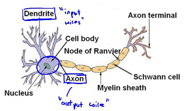
为了构建神经网络模型,我们需要借鉴大脑中的神经系统。每一个神经元都可以作为一个处理单元(Processing Unit)或神经核(Nucleus),其拥有众多用于输入的树突(Dendrite)和用于输出的轴突(Axon),其中神经元通过传递电脉冲来传递信息。
神经网络模型由一个个“神经元”构成,而每一个“神经元”又为一个学习模型,我们将这些“神经元”称为激活单元(Activation Unit)。

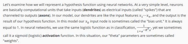
其中,参数θ在神经网络中也被称为权重,假设函数hθ(x) = g(z),新增的x0称为偏置单元(Bias Unit)。
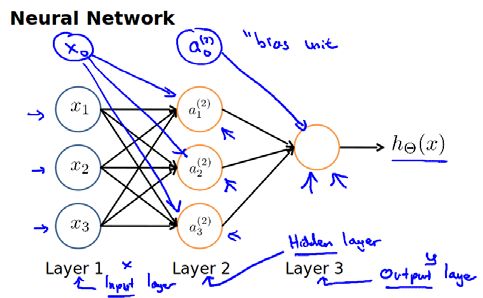
在神经网络模型中(以三层神经网络模型为例),第一层为输入层(Input Layer),最后一层为输出层(Output Layer),中间的这层称为隐藏层(Hidden Layer)。

我们引入如下标记用于描述神经网络模型:
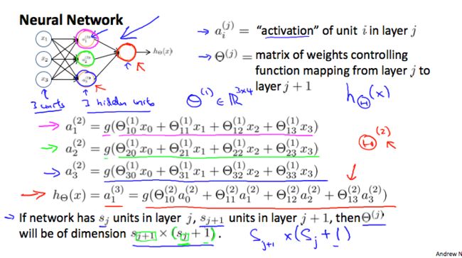
- ai(j):表示第j层的第i个激活单元;
- θ(j):表示从第j层映射到第j+1层时权重矩阵。
注:在神经网络模型中,如若第j层有sj个激活单元,在第j+1层有sj+1个激活单元,则权重矩阵θ(j)的维度为sj+1 * (sj+1)。因此,上图中权重矩阵θ(1)的维度3*4。
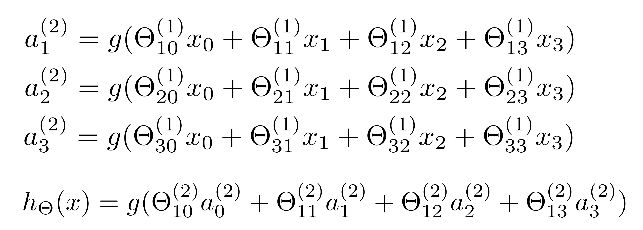
对于上图所示的神经网络模型,我们可用如下数学表达式表示:
在逻辑回归中,我们被限制使用数据集中的原始特征变量x,虽然我们可以通过多项式来组合这些特征,但我们仍然受到原始特征变量x的限制。
在神经网络中,原始特征变量x只作为输入层,输出层所做出的预测结果利用的是隐藏层的特征变量,由此我们可以认为隐藏层中特征变量是通过神经网络模型学习后,将得到的新特征用于预测结果,而非使用原始特征变量x用于预测结果。
补充笔记
Model Representation I
Visually, a simplistic representation looks like:

Our input nodes (layer 1), also known as the "input layer", go into another node (layer 2), which finally outputs the hypothesis function, known as the "output layer".
We can have intermediate layers of nodes between the input and output layers called the "hidden layers."
In this example, we label these intermediate or "hidden" layer nodes a02⋯an2 and call them "activation units."

If we had one hidden layer, it would look like:

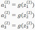
The values for each of the "activation" nodes is obtained as follows:

This is saying that we compute our activation nodes by using a 3×4 matrix of parameters. We apply each row of the parameters to our inputs to obtain the value for one activation node. Our hypothesis output is the logistic function applied to the sum of the values of our activation nodes, which have been multiplied by yet another parameter matrix Θ(2) containing the weights for our second layer of nodes.
Each layer gets its own matrix of weights, Θ(j).
The dimensions of these matrices of weights is determined as follows:
If network has sj units in layer j and sj+1 units in layer j+1, then Θ(j) will be of dimension sj+1×(sj+1).
The +1 comes from the addition in Θ(j) of the "bias nodes," x0 and Θ0(j). In other words the output nodes will not include the bias nodes while the inputs will. The following image summarizes our model representation:
模型表达Ⅱ(Model Representation II)
以此图为例,之前我们介绍其数学表达式。为了方便编码及运算,我们将其向量化。
其中:
因此,我们可将之前的数学表达式改写为:

其中向量X可记为a(1),则z(2) = Θ(1)a(1)。由此可得,a(2) = g(z(2))。
此时假设函数hθ(x)可改写为:
其中:
补充笔记
Model Representation II
To re-iterate, the following is an example of a neural network:

In this section we'll do a vectorized implementation of the above functions. We're going to define a new variable zk(j) that encompasses the parameters inside our g function. In our previous example if we replaced by the variable z for all the parameters we would get:
In other words, for layer j=2 and node k, the variable z will be:
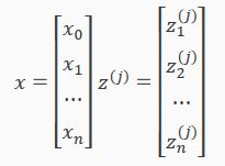
The vector representation of x and zj is:

Setting x=a(1), we can rewrite the equation as:
We are multiplying our matrix Θ(j−1) with dimensions sj×(n+1) (where sj is the number of our activation nodes) by our vector a(j−1) with height (n+1). This gives us our vector z(j) with height sj. Now we can get a vector of our activation nodes for layer j as follows:
Where our function g can be applied element-wise to our vector z(j).
We can then add a bias unit (equal to 1) to layer j after we have computed a(j). This will be element a0(j) and will be equal to 1. To compute our final hypothesis, let's first compute another z vector:
We get this final z vector by multiplying the next theta matrix after Θ(j−1) with the values of all the activation nodes we just got. This last theta matrix Θ(j) will have only one row which is multiplied by one column a(j) so that our result is a single number. We then get our final result with:
Notice that in this last step, between layer j and layer j+1, we are doing exactly the same thing as we did in logistic regression. Adding all these intermediate layers in neural networks allows us to more elegantly produce interesting and more complex non-linear hypotheses.