基于tensorflow2的VAE（mnist的生成）

Copyright 2018 The TensorFlow Authors.

#@title Licensed under the Apache License, Version 2.0 (the "License");
# you may not use this file except in compliance with the License.
# You may obtain a copy of the License at
#
# https://www.apache.org/licenses/LICENSE-2.0
#
# Unless required by applicable law or agreed to in writing, software
# distributed under the License is distributed on an "AS IS" BASIS,
# WITHOUT WARRANTIES OR CONDITIONS OF ANY KIND, either express or implied.
# See the License for the specific language governing permissions and
# limitations under the License.

Convolutional Variational Autoencoder

View on TensorFlow.org

Run in Google Colab

View source on GitHub

Download notebook

[外链图片转存失败,源站可能有防盗链机制,建议将图片保存下来直接上传(img-RPjkT2iQ-1591024661272)(https://tensorflow.org/images/autoencoders/cvae.gif)]

This notebook demonstrates how to generate images of handwritten digits by training a Variational Autoencoder (1, 2).

# to generate gifs
!pip install -q imageio

Import TensorFlow and other libraries

import tensorflow as tf

import os
import time
import numpy as np
import glob
import matplotlib.pyplot as plt
import PIL
import imageio

from IPython import display

Load the MNIST dataset

Each MNIST image is originally a vector of 784 integers, each of which is between 0-255 and represents the intensity of a pixel. We model each pixel with a Bernoulli distribution in our model, and we statically binarize the dataset.

(train_images, _), (test_images, _) = tf.keras.datasets.mnist.load_data()

train_images = train_images.reshape(train_images.shape[0], 28, 28, 1).astype('float32')
test_images = test_images.reshape(test_images.shape[0], 28, 28, 1).astype('float32')

# Normalizing the images to the range of [0., 1.]
train_images /= 255.
test_images /= 255.

# Binarization
train_images[train_images >= .5] = 1.
train_images[train_images < .5] = 0.
test_images[test_images >= .5] = 1.
test_images[test_images < .5] = 0.

TRAIN_BUF = 60000
BATCH_SIZE = 100

TEST_BUF = 10000

Use tf.data to create batches and shuffle the dataset

train_dataset = tf.data.Dataset.from_tensor_slices(train_images).shuffle(TRAIN_BUF).batch(BATCH_SIZE)
test_dataset = tf.data.Dataset.from_tensor_slices(test_images).shuffle(TEST_BUF).batch(BATCH_SIZE)

Wire up the generative and inference network with tf.keras.Sequential

In our VAE example, we use two small ConvNets for the generative and inference network. Since these neural nets are small, we use tf.keras.Sequential to simplify our code. Let $x$ and $z$ denote the observation and latent variable respectively in the following descriptions.

Generative Network

This defines the generative model which takes a latent encoding as input, and outputs the parameters for a conditional distribution of the observation, i.e. $p(x|z)$. Additionally, we use a unit Gaussian prior $p(z)$ for the latent variable.

Inference Network

This defines an approximate posterior distribution $q(z|x)$, which takes as input an observation and outputs a set of parameters for the conditional distribution of the latent representation. In this example, we simply model this distribution as a diagonal Gaussian. In this case, the inference network outputs the mean and log-variance parameters of a factorized Gaussian (log-variance instead of the variance directly is for numerical stability).

Reparameterization Trick

During optimization, we can sample from $q(z|x)$ by first sampling from a unit Gaussian, and then multiplying by the standard deviation and adding the mean. This ensures the gradients could pass through the sample to the inference network parameters.

Network architecture

For the inference network, we use two convolutional layers followed by a fully-connected layer. In the generative network, we mirror this architecture by using a fully-connected layer followed by three convolution transpose layers (a.k.a. deconvolutional layers in some contexts). Note, it’s common practice to avoid using batch normalization when training VAEs, since the additional stochasticity due to using mini-batches may aggravate instability on top of the stochasticity from sampling.

class CVAE(tf.keras.Model):
  def __init__(self, latent_dim):
    super(CVAE, self).__init__()
    self.latent_dim = latent_dim
    self.inference_net = tf.keras.Sequential(
      [
          tf.keras.layers.InputLayer(input_shape=(28, 28, 1)),
          tf.keras.layers.Conv2D(
              filters=32, kernel_size=3, strides=(2, 2), activation='relu'),
          tf.keras.layers.Conv2D(
              filters=64, kernel_size=3, strides=(2, 2), activation='relu'),
          tf.keras.layers.Flatten(),
          # No activation
          tf.keras.layers.Dense(latent_dim + latent_dim),
      ]
    )

    self.generative_net = tf.keras.Sequential(
        [
          tf.keras.layers.InputLayer(input_shape=(latent_dim,)),
          tf.keras.layers.Dense(units=7*7*32, activation=tf.nn.relu),
          tf.keras.layers.Reshape(target_shape=(7, 7, 32)),
          tf.keras.layers.Conv2DTranspose(
              filters=64,
              kernel_size=3,
              strides=(2, 2),
              padding="SAME",
              activation='relu'),
          tf.keras.layers.Conv2DTranspose(
              filters=32,
              kernel_size=3,
              strides=(2, 2),
              padding="SAME",
              activation='relu'),
          # No activation
          tf.keras.layers.Conv2DTranspose(
              filters=1, kernel_size=3, strides=(1, 1), padding="SAME"),
        ]
    )

  @tf.function
  def sample(self, eps=None):
    if eps is None:
      eps = tf.random.normal(shape=(100, self.latent_dim))
    return self.decode(eps, apply_sigmoid=True)

  def encode(self, x):
    mean, logvar = tf.split(self.inference_net(x), num_or_size_splits=2, axis=1)
    return mean, logvar

  def reparameterize(self, mean, logvar):
    eps = tf.random.normal(shape=mean.shape)
    return eps * tf.exp(logvar * .5) + mean

  def decode(self, z, apply_sigmoid=False):
    logits = self.generative_net(z)
    if apply_sigmoid:
      probs = tf.sigmoid(logits)
      return probs

    return logits

Define the loss function and the optimizer

VAEs train by maximizing the evidence lower bound (ELBO) on the marginal log-likelihood:

$$\log p(x)\ge \text{ELBO}={\mathbb{E}}_{q(z|x)}\left[\log \frac{p(x,z)}{q(z|x)}\right].$$

In practice, we optimize the single sample Monte Carlo estimate of this expectation:

$$\log p(x|z)+\log p(z)-\log q(z|x),$$
where $z$ is sampled from $q(z|x)$.

Note: we could also analytically compute the KL term, but here we incorporate all three terms in the Monte Carlo estimator for simplicity.

optimizer = tf.keras.optimizers.Adam(1e-4)

def log_normal_pdf(sample, mean, logvar, raxis=1):
  log2pi = tf.math.log(2. * np.pi)
  return tf.reduce_sum(
      -.5 * ((sample - mean) ** 2. * tf.exp(-logvar) + logvar + log2pi),
      axis=raxis)

@tf.function
def compute_loss(model, x):
  mean, logvar = model.encode(x)
  z = model.reparameterize(mean, logvar)
  x_logit = model.decode(z)

  cross_ent = tf.nn.sigmoid_cross_entropy_with_logits(logits=x_logit, labels=x)
  logpx_z = -tf.reduce_sum(cross_ent, axis=[1, 2, 3])
  logpz = log_normal_pdf(z, 0., 0.)
  logqz_x = log_normal_pdf(z, mean, logvar)
  return -tf.reduce_mean(logpx_z + logpz - logqz_x)

@tf.function
def compute_apply_gradients(model, x, optimizer):
  with tf.GradientTape() as tape:
    loss = compute_loss(model, x)
  gradients = tape.gradient(loss, model.trainable_variables)
  optimizer.apply_gradients(zip(gradients, model.trainable_variables))

Training

• We start by iterating over the dataset
• During each iteration, we pass the image to the encoder to obtain a set of mean and log-variance parameters of the approximate posterior $q(z|x)$
• We then apply the reparameterization trick to sample from $q(z|x)$
• Finally, we pass the reparameterized samples to the decoder to obtain the logits of the generative distribution $p(x|z)$
• Note: Since we use the dataset loaded by keras with 60k datapoints in the training set and 10k datapoints in the test set, our resulting ELBO on the test set is slightly higher than reported results in the literature which uses dynamic binarization of Larochelle’s MNIST.

Generate Images

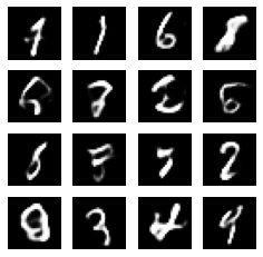
• After training, it is time to generate some images
• We start by sampling a set of latent vectors from the unit Gaussian prior distribution $p(z)$
• The generator will then convert the latent sample $z$ to logits of the observation, giving a distribution $p(x|z)$
• Here we plot the probabilities of Bernoulli distributions

epochs = 100
latent_dim = 50
num_examples_to_generate = 16

# keeping the random vector constant for generation (prediction) so
# it will be easier to see the improvement.
random_vector_for_generation = tf.random.normal(
    shape=[num_examples_to_generate, latent_dim])
model = CVAE(latent_dim)

def generate_and_save_images(model, epoch, test_input):
  predictions = model.sample(test_input)
  fig = plt.figure(figsize=(4,4))

  for i in range(predictions.shape[0]):
      plt.subplot(4, 4, i+1)
      plt.imshow(predictions[i, :, :, 0], cmap='gray')
      plt.axis('off')

  # tight_layout minimizes the overlap between 2 sub-plots
  plt.savefig('image_at_epoch_{:04d}.png'.format(epoch))
  plt.show()

generate_and_save_images(model, 0, random_vector_for_generation)

for epoch in range(1, epochs + 1):
  start_time = time.time()
  for train_x in train_dataset:
    compute_apply_gradients(model, train_x, optimizer)
  end_time = time.time()

  if epoch % 1 == 0:
    loss = tf.keras.metrics.Mean()
    for test_x in test_dataset:
      loss(compute_loss(model, test_x))
    elbo = -loss.result()
    display.clear_output(wait=False)
    print('Epoch: {}, Test set ELBO: {}, '
          'time elapse for current epoch {}'.format(epoch,
                                                    elbo,
                                                    end_time - start_time))
    generate_and_save_images(
        model, epoch, random_vector_for_generation)

Epoch: 100, Test set ELBO: -77.99336242675781, time elapse for current epoch 4.503999948501587

Display an image using the epoch number

def display_image(epoch_no):
  return PIL.Image.open('image_at_epoch_{:04d}.png'.format(epoch_no))

plt.imshow(display_image(epochs))
plt.axis('off')# Display images

(-0.5, 287.5, 287.5, -0.5)

Generate a GIF of all the saved images.

anim_file = 'cvae.gif'

with imageio.get_writer(anim_file, mode='I') as writer:
  filenames = glob.glob('image*.png')
  filenames = sorted(filenames)
  last = -1
  for i,filename in enumerate(filenames):
    frame = 2*(i**0.5)
    if round(frame) > round(last):
      last = frame
    else:
      continue
    image = imageio.imread(filename)
    writer.append_data(image)
  image = imageio.imread(filename)
  writer.append_data(image)

import IPython
if IPython.version_info >= (6,2,0,''):
  display.Image(filename=anim_file)

If you’re working in Colab you can download the animation with the code below:

try:
  from google.colab import files
except ImportError:
   pass
else:
  files.download(anim_file)