MATLAB 绘图之科技论文常用的数据可视化
MATLAB 绘图之科技论文常用的数据可视化
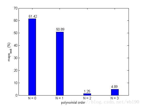
单柱状图
代码:
%%
clc; clear all; close all;
%%
x = [61.42 50.89 1.25 4.89];
b = bar(x,0.27,'b')
for i = 1:length(x)
    text(i-0.12, x(i)+2.0, num2str(x(i)))
end
ch = get(b, 'children')
set(gca, 'XTickLabel',{'N = 0', 'N = 1', 'N = 2', 'N = 3'})
xlabel('polynomial order')
ylabel('mape_{test} (%)')
输出:
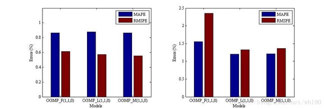
组柱状图
代码:
clc; clear all; close all
%%
train = [0.8646     0.8784  0.8626
         0.6135     0.5728  0.5528 ]';
test = [1.5566  1.2035  1.2163
        2.3511  1.3273  1.3609]';
%% Figure 2
figure (2)
subplot(121)
bar(train,'grouped') % 将train按照列分组 为 2 组
xlabel('Models','FontName', 'Times New Roman','FontSize', 9)
ylabel('Errors (%)','FontName', 'Times New Roman','FontSize', 9)
ylim([0 1.2])
legend('MAPE','RMSPE')
set(gca, 'FontName', 'Times New Roman','FontSize', 9, ...
    'XTickLabel',{'OGMP_F(1,1,0)', 'OGMP_L(1,1,0)', 'OGMP_M(1,1,0)'})

subplot(122)
bar(test,'grouped')
xlabel('Models','FontName', 'Times New Roman','FontSize', 9)
ylabel('Errors (%)','FontName', 'Times New Roman','FontSize', 9)
ylim([0 2.5])
legend('MAPE','RMSPE')
set(gca, 'FontName', 'Times New Roman','FontSize', 9, ...
    'XTickLabel',{'OGMP_F(1,1,0)', 'OGMP_L(1,1,0)', 'OGMP_M(1,1,0)'})
输出:
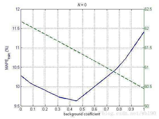
两个纵坐标轴
数据局部预览:
| 0.00 | 0.00 | -0.06 | 10.28 | 62.18 |
|---|---|---|---|---|
| 0.00 | 0.01 | -0.06 | 10.26 | 62.16 |
| 0.00 | 0.02 | -0.06 | 10.23 | 62.15 |
| 0.00 | 0.03 | -0.06 | 10.21 | 62.13 |
| 0.00 | 0.04 | -0.06 | 10.18 | 62.11 |
| 0.00 | 0.05 | -0.06 | 10.16 | 62.10 |
| 0.00 | 0.06 | -0.06 | 10.13 | 62.08 |
| 0.00 | 0.07 | -0.06 | 10.11 | 62.06 |
| 0.00 | 0.08 | -0.06 | 10.08 | 62.05 |
| polyOrder | baCoe | devCoe | mapeTrain | mapeTest |
代码:
gmpb = xlsread('GMPB_0.csv');
bc = gmpb(:,2); % X轴对应的数值
[haxes, hline1, hline2] = plotyy(bc, gmpb(:,4), bc, gmpb(:,5)); % gmpb(:,4) 左Y对应的数值, gmpb(:,5) 右Y对应的数值
grid on
xlabel('background coefficient'); ylabel('MAPE_{train} (%)')
axes(haxes(1)); set(hline1,'LineStyle','-','LineWidth',2);
axes(haxes(2)); set(hline2,'LineStyle','--','LineWidth',2)
title('\it{N} \rm{= 0}');
输出:
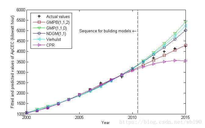
数据划分与标注
数据局部预览:
| 2000 | 1066.9 | 1068.3 | 1040.2 | 1066.9 | 1066.9 | 1055.6 |
|---|---|---|---|---|---|---|
| 2001 | 1157.6 | 1149.7 | 1228.3 | 1147.2 | 1195.2 | 1158.7 |
| 2002 | 1286.0 | 1292.6 | 1365.7 | 1315.7 | 1357.8 | 1304.8 |
| 2003 | 1477.1 | 1484.7 | 1518.4 | 1496.4 | 1525.2 | 1485.8 |
| 2004 | 1695.2 | 1700.4 | 1688.2 | 1690.1 | 1703.9 | 1694.2 |
| 2005 | 1913.0 | 1927.6 | 1877.1 | 1897.8 | 1897.3 | 1922.0 |
| 2006 | 2180.6 | 2160.2 | 2087.0 | 2120.5 | 2108.2 | 2161.5 |
| Year | Consumption | GMPB(1,1,2) | GMP(1,1,0) | NDGM(1,1) | Verhulst | CPR |
代码:
clc; clear all; close all;
%%
[gmp,txt,raw] = xlsread('对比模型结果.xlsx');
t = gmp(:,1);
%%
figure (4)
plot(t, gmp(:,2),'+k','LineWidth',2); hold on
plot(t, gmp(:,3),'-rs','LineWidth',1);
plot(t, gmp(:,4),'-gv','LineWidth',1);
plot(t, gmp(:,5),'-bo','LineWidth',1);
plot(t, gmp(:,6),'-c<','LineWidth',1);
plot(t, gmp(:,7),'-m>','LineWidth',1);
legend('Actual values', 'GMPB(1,1,2)', 'GMP(1,1,0)', 'NDGM(1,1)', 'Verhulst', 'CPR')
plot([2010.5 2010.5], [1000 6000], 'k--')
text(2005, 5000, 'Sequence for buliding models \leftarrow ')
% text(2010, 5000, '\rightarrow Testing sequence')
xlabel('Year')
ylabel('Fitted and predicted values of ApCEC (kilowatt hour)')
hold off
输出:
数学公式的表述
示例代码:
xlabel('$$k$$','interpreter', 'latex', 'FontName', 'Cambria', 'FontSize', 12)
ylabel('$$\delta^{(r)}(k)$$','interpreter', 'latex', 'FontName', 'Cambria', 'FontSize', 12)
指定标注形状及颜色
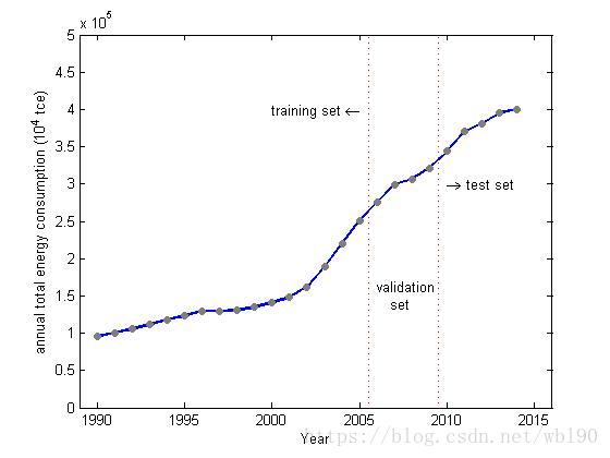
代码:
t = 1990:2014;
cvc = [95384 100413 105602 111490 118071 123471 129665 130082 ...
    130260 135132 140993 148264 161935 189269 220738 250835 ...
    275134 299271 306455 321336 343601 370163 381515 394794 400299];
plot(t, cvc, '-bo', 'Linewidth', 1.5, ...
    'MarkerEdgeColor',[.5 .5 .5], 'MarkerFaceColor',[.5 .5 .5], 'MarkerSize',5)
hold on
plot(2005.5*[1 1], 5*10^5*[0 1], ':r', 'Linewidth', 1)
text(2000, 4*10^5, 'training set \leftarrow ') % training set
plot(2009.5*[1 1], 5*10^5*[0 1], ':r', 'Linewidth', 1)
text(2010, 3*10^5, '\rightarrow test set') % test set
textstr={'validation'; '   set'}; % validation set
text(2006, 1.5*10^5, textstr)
% text(2005.8, 1.5*10^5, '\rightarrow') % validation set
% text(2008.5, 1*10^5, '\leftarrow') % validation set
hold off
xlim([1989 2016])
xlabel('Year'); ylabel('annual total energy consumption (10^4 tce)')
输出:
图形局部放大
数据局部预览:
| 0.02 | 58.98411 | 53607.07 |
|---|---|---|
| 0.04 | 18.23699 | 14261.72 |
| 0.06 | 11.37505 | 6999.15 |
| 0.08 | 9.809482 | 4481.429 |
| 0.1 | 10.01344 | 3338.315 |
| 0.12 | 11.10905 | 2736.983 |
| 0.14 | 12.79261 | 2391.725 |
| 0.16 | 14.93703 | 2183.315 |
| 0.18 | 17.48202 | 2055.052 |
| rho | condnum_0 | condnum_1 |
代码:
clc; clear all; close all
%%
condnum = xlsread('condnum.csv');
rho = condnum(:,1); condnum_0 = condnum(:,2); condnum_1 = condnum(:,3);
%% 绘图
figure (1)
%
subplot(121)
plot(rho, condnum_0, '-bo', 'LineWidth',1.5, ...
    'MarkerEdgeColor',[.5 .5 .5], 'MarkerFaceColor',[.5 .5 .5], 'MarkerSize',5)
xlabel('multiple coefficient'); ylabel('condition number')
axes('position', [0.17 0.58, 0.20, 0.30])
plot(rho, condnum_0, '-bo', 'LineWidth',1.5, ...
    'MarkerEdgeColor',[.5 .5 .5], 'MarkerFaceColor',[.5 .5 .5], 'MarkerSize',5); grid on; xlim([0.04 0.44])
%
subplot(122)
plot(rho, condnum_1, '-bo', 'LineWidth',1.5, ...
    'MarkerEdgeColor',[.5 .5 .5], 'MarkerFaceColor',[.5 .5 .5], 'MarkerSize',5)
xlabel('multiple coefficient'); ylabel('condition number')
axes('position', [0.67 0.58, 0.20, 0.30])
plot(rho, condnum_1, '-bo', 'LineWidth',1.5, ...
    'MarkerEdgeColor',[.5 .5 .5], 'MarkerFaceColor',[.5 .5 .5], 'MarkerSize',5); grid on; xlim([0.04 0.44])
输出:
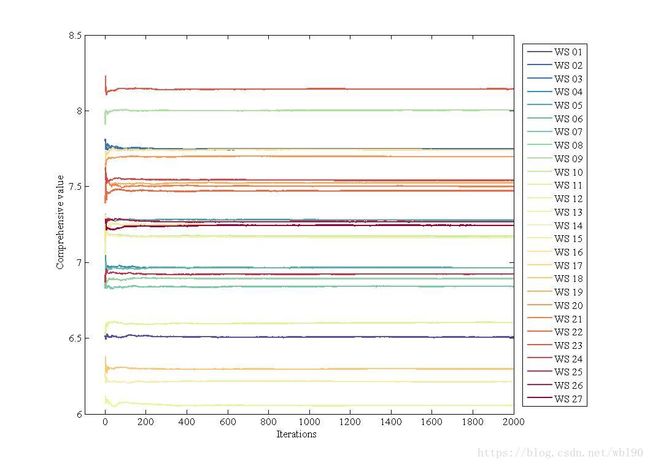
多种线指定颜色
数据局预览:
| WS1 | WS2 | WS3 | WS4 | WS5 | WS6 | WS7 | WS8 | WS9 | WS10 | WS11 | WS12 | WS13 | WS14 | WS15 | WS16 | WS17 | WS18 | WS19 | WS20 | WS21 | WS22 | WS23 | WS24 | WS25 | WS26 | WS27 |
|---|---|---|---|---|---|---|---|---|---|---|---|---|---|---|---|---|---|---|---|---|---|---|---|---|---|---|
| 6.5076 | 7.8022 | 7.7834 | 7.0455 | 7.3199 | 6.9144 | 6.8269 | 6.8670 | 7.9091 | 7.1654 | 6.5740 | 6.1191 | 7.0559 | 7.2718 | 6.2431 | 7.1305 | 7.7343 | 6.3780 | 7.5796 | 7.6400 | 7.3905 | 7.5288 | 8.2310 | 7.6288 | 6.8708 | 7.2760 | 7.2873 |
| 6.5155 | 7.8143 | 7.7859 | 6.9928 | 7.2758 | 6.8948 | 6.8826 | 6.8882 | 7.9830 | 7.2577 | 6.5203 | 6.1160 | 7.1873 | 7.3162 | 6.2738 | 7.2242 | 7.6861 | 6.3770 | 7.5720 | 7.6093 | 7.4405 | 7.5138 | 8.1840 | 7.6233 | 6.9131 | 7.2788 | 7.2710 |
| 6.4982 | 7.7506 | 7.7432 | 6.9282 | 7.2679 | 6.9143 | 6.8457 | 6.9024 | 8.0037 | 7.2444 | 6.5697 | 6.0754 | 7.1706 | 7.3010 | 6.2063 | 7.2102 | 7.6665 | 6.2826 | 7.5757 | 7.6348 | 7.4445 | 7.4742 | 8.1369 | 7.5665 | 6.9245 | 7.2797 | 7.2716 |
| 6.4943 | 7.7628 | 7.7578 | 6.9601 | 7.2506 | 7.0064 | 6.8726 | 6.8923 | 7.9948 | 7.2165 | 6.5543 | 6.0697 | 7.1794 | 7.2889 | 6.2130 | 7.1872 | 7.6989 | 6.2774 | 7.5694 | 7.6466 | 7.4483 | 7.4294 | 8.1152 | 7.5429 | 6.9220 | 7.2874 | 7.2611 |
| 6.5087 | 7.7649 | 7.7713 | 6.9814 | 7.2873 | 6.9648 | 6.8611 | 6.8873 | 7.9984 | 7.2308 | 6.5813 | 6.0781 | 7.2037 | 7.2731 | 6.2221 | 7.1958 | 7.7296 | 6.2837 | 7.5700 | 7.6510 | 7.5240 | 7.4228 | 8.1108 | 7.5496 | 6.9302 | 7.2661 | 7.2566 |
| 6.5094 | 7.7583 | 7.7667 | 6.9761 | 7.2850 | 6.9620 | 6.8364 | 6.8701 | 8.0017 | 7.2316 | 6.6012 | 6.0971 | 7.2224 | 7.2825 | 6.2135 | 7.2095 | 7.7289 | 6.2793 | 7.5655 | 7.6758 | 7.5385 | 7.4141 | 8.1063 | 7.5226 | 6.9389 | 7.2603 | 7.2147 |
| 6.5118 | 7.7533 | 7.7660 | 6.9784 | 7.2911 | 6.9437 | 6.8403 | 6.8651 | 8.0017 | 7.2291 | 6.5939 | 6.0849 | 7.2298 | 7.2867 | 6.2191 | 7.2231 | 7.7169 | 6.2797 | 7.5430 | 7.6801 | 7.5275 | 7.4240 | 8.1094 | 7.5467 | 6.9580 | 7.2684 | 7.2202 |
| 6.5234 | 7.7502 | 7.7635 | 6.9641 | 7.2964 | 6.9412 | 6.8287 | 6.8743 | 7.9938 | 7.2136 | 6.5883 | 6.0748 | 7.2133 | 7.2877 | 6.2450 | 7.2367 | 7.7102 | 6.2732 | 7.5429 | 7.6707 | 7.5383 | 7.4190 | 8.1104 | 7.5562 | 6.9545 | 7.2704 | 7.2258 |
代码:
clear all; close all; clc
%%
X = xlsread('5000iterationsCumsmeanMeasure.xlsx');
X = X(1:2000,:);
[m, n] = size(X);
t = (1:m)';
%%
figure (1)
C = linspecer(n);
for i=1:n
    plot(X(:,i), 'color', C(i,:), 'linewidth', 2);
    hold on
end
xlim([-100 2000])
xlabel('Iterations ', 'FontName', 'Times New Roman', 'FontSize', 12)
ylabel('Comprehensive value', 'FontName', 'Times New Roman', 'FontSize', 12)
set(gca, 'FontName', 'Times New Roman', 'FontSize', 12)
hleg = legend('WS 01','WS 02','WS 03', 'WS 04','WS 05','WS 06','WS 07','WS 08','WS 09','WS 10',...
            'WS 11','WS 12','WS 13', 'WS 14','WS 15','WS 16','WS 17','WS 18','WS 19','WS 20',...
            'WS 21','WS 22','WS 23', 'WS 24','WS 25','WS 26','WS 27', 'FontSize', 8, 'Location','EastOutside') %
hold off
输出:
特别注意: 在当前工作目录下添加 ‘function’ 文件(linspecer.m)
% function lineStyles = linspecer(N)
% This function creates an Nx3 array of N [R B G] colors
% These can be used to plot lots of lines with distinguishable and nice
% looking colors.
%
% lineStyles = linspecer(N);  makes N colors for you to use: lineStyles(ii,:)
%
% colormap(linspecer); set your colormap to have easily distinguishable
%                      colors and a pleasing aesthetic
%
% lineStyles = linspecer(N,'qualitative'); forces the colors to all be distinguishable (up to 12)
% lineStyles = linspecer(N,'sequential'); forces the colors to vary along a spectrum
%
% % Examples demonstrating the colors.
%
% LINE COLORS
% N=6;
% X = linspace(0,pi*3,1000);
% Y = bsxfun(@(x,n)sin(x+2*n*pi/N), X.', 1:N);
% C = linspecer(N);
% axes('NextPlot','replacechildren', 'ColorOrder',C);
% plot(X,Y,'linewidth',5)
% ylim([-1.1 1.1]);
%
% SIMPLER LINE COLOR EXAMPLE
% N = 6; X = linspace(0,pi*3,1000);
% C = linspecer(N)
% hold off;
% for ii=1:N
%     Y = sin(X+2*ii*pi/N);
%     plot(X,Y,'color',C(ii,:),'linewidth',3);
%     hold on;
% end
%
% COLORMAP EXAMPLE
% A = rand(15);
% figure; imagesc(A); % default colormap
% figure; imagesc(A); colormap(linspecer); % linspecer colormap
%
%%%%%%%%%%%%%%%%%%%%%%%%%%%%%%%%%%%%%%%%%%%%%%%%%%%%%%%%%%%%%%%%%%%%%%%%%%%
% by Jonathan Lansey, March 2009-2013 �Lansey at gmail.com               %
%%%%%%%%%%%%%%%%%%%%%%%%%%%%%%%%%%%%%%%%%%%%%%%%%%%%%%%%%%%%%%%%%%%%%%%%%%%
%
%% credits and where the function came from
% The colors are largely taken from:
% http://colorbrewer2.org and Cynthia Brewer, Mark Harrower and The Pennsylvania State University
%
%
% She studied this from a phsychometric perspective and crafted the colors
% beautifully.
%
% I made choices from the many there to decide the nicest once for plotting
% lines in Matlab. I also made a small change to one of the colors I
% thought was a bit too bright. In addition some interpolation is going on
% for the sequential line styles.
%
%
%%

function lineStyles=linspecer(N,varargin)

if nargin==0 % return a colormap
    lineStyles = linspecer(64);
%     temp = [temp{:}];
%     lineStyles = reshape(temp,3,255)';
    return;
end

if N<=0 % its empty, nothing else to do here
    lineStyles=[];
    return;
end

% interperet varagin
qualFlag = 0;

if ~isempty(varargin)>0 % you set a parameter?
    switch lower(varargin{1})
        case {'qualitative','qua'}
            if N>12 % go home, you just can't get this.
                warning('qualitiative is not possible for greater than 12 items, please reconsider');
            else
                if N>9
                    warning(['Default may be nicer for ' num2str(N) ' for clearer colors use: whitebg(''black''); ']);
                end
            end
            qualFlag = 1;
        case {'sequential','seq'}
            lineStyles = colorm(N);
            return;
        otherwise
            warning(['parameter ''' varargin{1} ''' not recognized']);
    end
end

% predefine some colormaps
  set3 = colorBrew2mat({[141, 211, 199];[ 255, 237, 111];[ 190, 186, 218];[ 251, 128, 114];[ 128, 177, 211];[ 253, 180, 98];[ 179, 222, 105];[ 188, 128, 189];[ 217, 217, 217];[ 204, 235, 197];[ 252, 205, 229];[ 255, 255, 179]}');
set1JL = brighten(colorBrew2mat({[228, 26, 28];[ 55, 126, 184];[ 77, 175, 74];[ 255, 127, 0];[ 255, 237, 111]*.95;[ 166, 86, 40];[ 247, 129, 191];[ 153, 153, 153];[ 152, 78, 163]}'));
set1 = brighten(colorBrew2mat({[ 55, 126, 184]*.95;[228, 26, 28];[ 77, 175, 74];[ 255, 127, 0];[ 152, 78, 163]}),.8);

set3 = dim(set3,.93);

switch N
    case 1
        lineStyles = { [  55, 126, 184]/255};
    case {2, 3, 4, 5 }
        lineStyles = set1(1:N);
    case {6 , 7, 8, 9}
        lineStyles = set1JL(1:N)';
    case {10, 11, 12}
        if qualFlag % force qualitative graphs
            lineStyles = set3(1:N)';
        else % 10 is a good number to start with the sequential ones.
            lineStyles = cmap2linspecer(colorm(N));
        end
otherwise % any old case where I need a quick job done.
    lineStyles = cmap2linspecer(colorm(N));
end
lineStyles = cell2mat(lineStyles);
end

% extra functions
function varIn = colorBrew2mat(varIn)
for ii=1:length(varIn) % just divide by 255
    varIn{ii}=varIn{ii}/255;
end
end

function varIn = brighten(varIn,varargin) % increase the brightness

if isempty(varargin),
    frac = .9;
else
    frac = varargin{1};
end

for ii=1:length(varIn)
    varIn{ii}=varIn{ii}*frac+(1-frac);
end
end

function varIn = dim(varIn,f)
    for ii=1:length(varIn)
        varIn{ii} = f*varIn{ii};
    end
end

function vOut = cmap2linspecer(vIn) % changes the format from a double array to a cell array with the right format
vOut = cell(size(vIn,1),1);
for ii=1:size(vIn,1)
    vOut{ii} = vIn(ii,:);
end
end
%%
% colorm returns a colormap which is really good for creating informative
% heatmap style figures.
% No particular color stands out and it doesn't do too badly for colorblind people either.
% It works by interpolating the data from the
% 'spectral' setting on http://colorbrewer2.org/ set to 11 colors
% It is modified a little to make the brightest yellow a little less bright.
function cmap = colorm(varargin)
n = 100;
if ~isempty(varargin)
    n = varargin{1};
end

if n==1
    cmap =  [0.2005    0.5593    0.7380];
    return;
end
if n==2
     cmap =  [0.2005    0.5593    0.7380;
              0.9684    0.4799    0.2723];
          return;
end

frac=.95; % Slight modification from colorbrewer here to make the yellows in the center just a bit darker
cmapp = [158, 1, 66; 213, 62, 79; 244, 109, 67; 253, 174, 97; 254, 224, 139; 255*frac, 255*frac, 191*frac; 230, 245, 152; 171, 221, 164; 102, 194, 165; 50, 136, 189; 94, 79, 162];
x = linspace(1,n,size(cmapp,1));
xi = 1:n;
cmap = zeros(n,3);
for ii=1:3
    cmap(:,ii) = pchip(x,cmapp(:,ii),xi);
end
cmap = flipud(cmap/255);
end