图神经网络的简要介绍（基础知识，DeepWalk和GraphSage）

A Gentle Introduction to Graph Neural Networks (Basics, DeepWalk, and GraphSage)

图神经网络的简要介绍（基础知识，DeepWalk和GraphSage）

Recently, Graph Neural Network (GNN) has gained increasing popularity in various domains, including social network, knowledge graph, recommender system, and even life science. The power of GNN in modeling the dependencies between nodes in a graph enables the breakthrough in the research area related to graph analysis. This article aims to introduce the basics of Graph Neural Network and two more advanced algorithms, DeepWalk and GraphSage.
最近，图形神经网络（GNN）在各种领域越来越受欢迎，包括社交网络，知识图，推荐系统，甚至生命科学。 GNN在对图中节点之间的依赖关系建模方面的强大功能使得与图分析相关的研究领域取得了突破。 本文旨在介绍图形神经网络的基础知识和两种更高级的算法，DeepWalk和GraphSage。

Graph

Before we get into GNN, let’s first understand what is Graph. In Computer Science, a graph is a data structure consisting of two components, vertices and edges. A graph G can be well described by the set of vertices V and edges E it contains.
在我们进入GNN之前，让我们先了解一下Graph是什么。 在计算机科学中，图形是由两个组成部分组成的数据结构，顶点和边缘。 图G可以通过顶点集V和它包含的边E来很好地描述。

Edges can be either directed or undirected, depending on whether there exist directional dependencies between vertices.
根据顶点之间是否存在方向依赖性，边缘可以是定向的或不定向的。

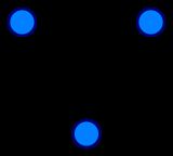
The vertices are often called nodes. In this article, these two terms are interchangeable.
顶点通常称为节点。 在本文中，这两个术语是可以互换的。

Graph Neural Network

Graph Neural Network is a type of Neural Network which directly operates on the Graph structure. A typical application of GNN is node classification. Essentially, every node in the graph is associated with a label, and we want to predict the label of the nodes without ground-truth. This section will illustrate the algorithm described in the paper, the first proposal of GNN and thus often regarded as the original GNN.

In the node classification problem setup, each node v is characterized by its feature x_v and associated with a ground-truth label t_v. Given a partially labeled graph G, the goal is to leverage these labeled nodes to predict the labels of the unlabeled. It learns to represent each node with a d dimensional vector (state) h_v which contains the information of its neighborhood. Specifically,
图神经网络是一种直接在图形结构上运行的神经网络。 GNN的典型应用是节点分类。 本质上，图中的每个节点都与一个标签相关联，我们希望预测没有地面实况的节点的标签。 本节将说明本文中描述的算法，GNN的第一个提议，因此通常被视为原始GNN。

在节点分类问题设置中，每个节点v的特征在于其特征x_v并且与地面实况标签t_v相关联。 给定部分标记的图G，目标是利用这些标记的节点来预测未标记的标记。 它学会用d维向量（状态）h_v表示每个节点，其中包含其邻域的信息。 特别，

where x_co[v] denotes the features of the edges connecting with v, h_ne[v] denotes the embedding of the neighboring nodes of v, and x_ne[v] denotes the features of the neighboring nodes of v. The function f is the transition function that projects these inputs onto a d-dimensional space. Since we are seeking a unique solution for h_v, we can apply Banach fixed point theorem and rewrite the above equation as an iteratively update process. Such operation is often referred to as message passing or neighborhood aggregation.
其中x_co [v]表示与v连接的边的特征，h_ne [v]表示嵌入v的相邻节点，x_ne [v]表示v的相邻节点的特征。函数f是转换 将这些输入投影到d维空间的函数。 由于我们正在寻找h_v的唯一解，我们可以应用Banach不动点定理并将上述等式重写为迭代更新过程。 这种操作通常被称为消息传递或邻居聚合。

H and X denote the concatenation of all the h and x, respectively.

The output of the GNN is computed by passing the state h_v as well as the feature x_v to an output function g.
H和X分别表示所有h和x的串联。

通过将状态h_v以及特征x_v传递给输出函数g来计算GNN的输出。

Both f and g here can be interpreted as feed-forward fully-connected Neural Networks. The L1 loss can be straightforwardly formulated as the following:
这里的f和g都可以解释为前馈全连接神经网络。 L1损失可以直接表述如下：

which can be optimized via gradient descent.

However, there are three main limitations with this original proposal of GNN pointed out by this paper:

If the assumption of “fixed point” is relaxed, it is possible to leverage Multi-layer Perceptron to learn a more stable representation, and removing the iterative update process. This is because, in the original proposal, different iterations use the same parameters of the transition function f, while the different parameters in different layers of MLP allow for hierarchical feature extraction.
It cannot process edge information (e.g. different edges in a knowledge graph may indicate different relationship between nodes)
Fixed point can discourage the diversification of node distribution, and thus may not be suitable for learning to represent nodes.
Several variants of GNN have been proposed to address the above issue. However, they are not covered as they are not the focus in this post.
可以通过梯度下降优化。

但是，本文指出的GNN原始提案有三个主要限制：

如果放宽了“固定点”的假设，则可以利用多层感知器来学习更稳定的表示，并删除迭代更新过程。 这是因为，在原始提议中，不同的迭代使用转移函数f的相同参数，而不同MLP层中的不同参数允许分层特征提取。
它不能处理边缘信息（例如，知识图中的不同边缘可能表示节点之间的不同关系）
固定点可以阻止节点分布的多样化，因此可能不适合学习表示节点。
已经提出了几种GNN变体来解决上述问题。 但是，他们没有被涵盖，因为他们不是这篇文章的重点。

DeepWalk

DeepWalk is the first algorithm proposing node embedding learned in an unsupervised manner. It highly resembles word embedding in terms of the training process. The motivation is that the distribution of both nodes in a graph and words in a corpus follow a power law as shown in the following figure:
DeepWalk是第一个提出以无人监督的方式学习的节点嵌入的算法。 它在培训过程中非常类似于字嵌入。 动机是图表中的两个节点和语料库中的单词的分布遵循幂律，如下图所示：

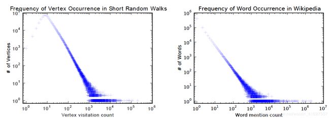
The algorithm contains two steps:

• 1 Perform random walks on nodes in a graph to generate node sequences
• 2 Run skip-gram to learn the embedding of each node based on the node sequences generated in step 1

At each time step of the random walk, the next node is sampled uniformly from the neighbor of the previous node. Each sequence is then truncated into sub-sequences of length 2|w| + 1, where w denotes the window size in skip-gram. If you are not familiar with skip-gram, my previous blog post shall brief you how it works.

In this paper, hierarchical softmax is applied to address the costly computation of softmax due to the huge number of nodes. To compute the softmax value of each of the individual output element, we must compute all the e^xk for all the element k.
该算法包含两个步骤：

• 1在图形中的节点上执行随机遍历以生成节点序列
• 2运行skip-gram，根据步骤1中生成的节点序列学习每个节点的嵌入

在随机游走的每个时间步骤，从前一节点的邻居统一采样下一个节点。 然后将每个序列截短为长度为2 | w |的子序列 + 1，其中w表示skip-gram中的窗口大小。 如果您不熟悉skip-gram，我之前的博客文章将向您介绍它的工作原理。

在本文中，分层softmax用于解决由于节点数量庞大而导致的softmax计算成本高昂的问题。 为了计算每个单独输出元素的softmax值，我们必须计算所有元素k的所有e ^ xk。

Therefore, the computation time is O(|V|) for the original softmax, where V denotes the set of vertices in the graph.

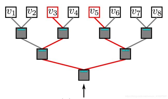
Hierarchical softmax utilizes a binary tree to deal with the problem. In this binary tree, all the leaves (v1, v2, … v8 in the above graph) are the vertices in the graph. In each of the inner node, there is a binary classifier to decide which path to choose. To compute the probability of a given vertex v_k, one simply compute the probability of each of the sub-path along the path from the root node to the leave v_k. Since the probability of each node’ children sums to 1, the property that the sum of the probability of all the vertices equals 1 still holds in the hierarchical softmax. The computation time for an element is now reduced to O(log|V|) as the longest path for a binary tree is bounded by O(log(n)) where n is the number of leaves.
因此，原始softmax的计算时间为O（| V |），其中V表示图中的顶点集。

分层softmax利用二叉树来处理问题。 在这个二叉树中，所有叶子（上图中的v1，v2，… v8）都是图中的顶点。 在每个内部节点中，有一个二元分类器来决定选择哪条路径。 为了计算给定顶点v_k的概率，可以简单地计算沿着从根节点到离开v_k的路径中的每个子路径的概率。 由于每个节点的子概率为1，因此所有顶点的概率之和等于1的特性仍然保持在分层softmax中。 现在，元素的计算时间减少到O（log | V |），因为二叉树的最长路径由O（log（n））限定，其中n是叶子的数量。

After a DeepWalk GNN is trained, the model has learned a good representation of each node as shown in the following figure. Different colors indicate different labels in the input graph. We can see that in the output graph (embedding with 2 dimensions), nodes having the same labels are clustered together, while most nodes with different labels are separated properly.
在训练DeepWalk GNN之后，模型已经学习了每个节点的良好表示，如下图所示。 不同的颜色表示输入图中的不同标签。 我们可以看到，在输出图（嵌入2维）中，具有相同标签的节点聚集在一起，而具有不同标签的大多数节点被正确分开。

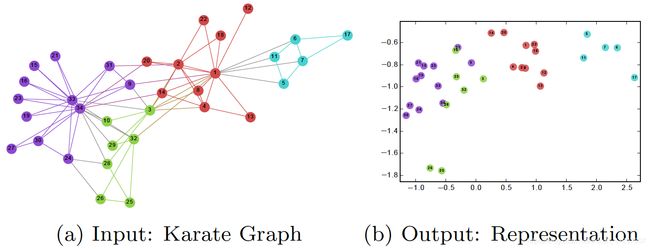
However, the main issue with DeepWalk is that it lacks the ability of generalization. Whenever a new node comes in, it has to re-train the model in order to represent this node (transductive). Thus, such GNN is not suitable for dynamic graphs where the nodes in the graphs are ever-changing.
然而，DeepWalk的主要问题是它缺乏泛化能力。 每当有新节点进入时，它必须重新训练模型以表示该节点（转换）。 因此，这种GNN不适用于图中节点不断变化的动态图。

GraphSage

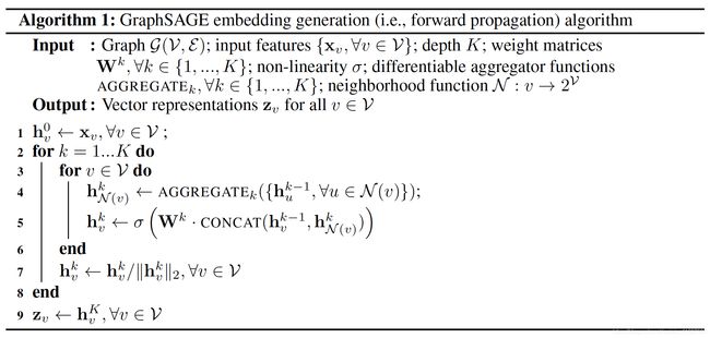
GraphSage provides a solution to address the aforementioned problem, learning the embedding for each node in an inductive way. Specifically, each node is represented by the aggregation of its neighborhood. Thus, even if a new node unseen during training time appears in the graph, it can still be properly represented by its neighboring nodes. Below shows the algorithm of GraphSage.
GraphSage提供解决上述问题的解决方案，以归纳方式学习每个节点的嵌入。 具体而言，每个节点由其邻域的聚合表示。 因此，即使在训练时间期间看不到的新节点出现在图中，它仍然可以由其相邻节点正确地表示。 下面显示了GraphSage的算法。

The outer loop indicates the number of update iteration, while h^k_v denotes the latent vector of node v at update iteration k. At each update iteration, h^k_v is updated based on an aggregation function, the latent vectors of v and v’s neighborhood in the previous iteration, and a weight matrix W^k. The paper proposed three aggregation function:
外环表示更新迭代次数，而h ^ k_v表示更新迭代k时节点v的潜在向量。 在每次更新迭代时，基于聚合函数，前一次迭代中v和v邻域的潜在向量以及权重矩阵W ^ k来更新h ^ k_v。 本文提出了三种聚合函数：

1. Mean aggregator:

The mean aggregator takes the average of the latent vectors of a node and all its neighborhood.
平均聚合器获取节点及其所有邻域的潜在向量的平均值。

Compared with the original equation, it removes the concatenation operation at line 5 in the above pseudo code. This operation can be viewed as a “skip-connection”, which later in the paper proved to largely improve the performance of the model.
与原始方程相比，它删除了上述伪代码中第5行的连接操作。 此操作可以被视为“跳过连接”，本文稍后将证明可以在很大程度上提高模型的性能。

2. LSTM aggregator:

Since the nodes in the graph don’t have any order, they assign the order randomly by permuting these nodes.
由于图中的节点没有任何顺序，因此它们通过置换这些节点来随机分配顺序。

3. Pooling aggregator:

This operator performs an element-wise pooling function on the neighboring set. Below shows an example of max-pooling:
此运算符在相邻集上执行逐元素池功能。 下面显示了最大池的示例：

, which can be replaced with mean-pooling or any other symmetric pooling function. It points out that pooling aggregator performs the best, while mean-pooling and max-pooling aggregator have similar performance. The paper uses max-pooling as the default aggregation function.

The loss function is defined as the following:
，可以用平均池或任何其他对称池函数替换。 它指出池聚合器执行最佳，而均值池和最大池聚合器具有相似的性能。 本文使用max-pooling作为默认聚合函数。

损失函数定义如下：

where u and v co-occur in a fixed-length random walk, while v_n are the negative samples that don’t co-occur with u. Such loss function encourages nodes closer to have similar embedding, while those far apart to be separated in the projected space. Via this approach, the nodes will gain more and more information about their neighborhoods.

GraphSage enables representable embedding to be generated for unseen nodes by aggregating its nearby nodes. It allows node embedding to be applied to domains involving dynamic graph, where the structure of the graph is ever-changing. Pinterest, for example, has adopted an extended version of GraphSage, PinSage, as the core of their content discovery system.
其中u和v共同出现在固定长度的随机游走中，而v_n是不与u共同出现的负样本。 这种损失函数鼓励节点更接近具有类似的嵌入，而那些相距很远的节点在投影空间中分离。 通过这种方法，节点将获得越来越多关于其邻域的信息。

GraphSage通过聚合其附近的节点，可以为看不见的节点生成可表示的嵌入。 它允许将节点嵌入应用于涉及动态图的域，其中图的结构不断变化。 例如，Pinterest采用了GraphSage的扩展版本，PinSage，作为其内容发现系统的核心。

Conclusion

You have learned the basics of Graph Neural Networks, DeepWalk, and GraphSage. The power of GNN in modeling complex graph structures is truly astonishing. In view of its effectiveness, I believe, in the near future, GNN will play an important role in AI’s development. If you like my article, don’t forget to follow me on Medium and Twitter, where I frequently shared the most advanced development of AI, ML, and DL.
您已经学习了图形神经网络，DeepWalk和GraphSage的基础知识。 GNN在复杂图形结构建模中的强大功能确实令人惊讶。 鉴于其有效性，我相信，在不久的将来，GNN将在人工智能的发展中发挥重要作用。 如果您喜欢我的文章，请不要忘记关注我，我经常分享AI，ML和DL的最高级开发文章与技术博客。