关系图卷积网络(Relational graph convolutional network, R-GCN)
关系图卷积网络(R-GCN)
这里,我们将会了解如何实现一个关系图卷积网络(R-GCN),这种类型的网络旨在泛化GCN来处理知识库中实体之间的不同关系。如果想要学习更多R-GCN背后的东西,可以看Modeling Relational Data with Graph Convolutional Networks
简单的图卷积网络(GCN)和DGL探索一个数据集的结构信息(即,图的连通性)来改善节点表示的提取。图的边被保留为无类型。
知识图由主题,关系,对象形式的三元组集合组成。 因此,边对重要信息进行编码,并具有自己有待学习的嵌入。 此外,在任何给定对之间可能存在多个边。
R-GCN的一个简单介绍
在统计关系学习(statistical relational learning, SRL)中,有两类基本任务:
- 实体分类——需要指定实体的类型和分类属性
- 链路预测——需要发现丢失的三元组
上面两种情况中,我们都期望可以从图的邻居结构中发现丢失的信息。例如,有一篇R-GCN的文章提供了下面的例子。在知道Mikhail Baryshnikov曾经在Vaganova Academy受教育,可以推断出Mikhail Baryshnikov是有标签的,而且我们也可以知道三元组(Mikhail Baryshnikov, lived in, Russia)一定属于这个知识图。
R-GCN通过一个常见的图卷积网络来解决上面两个问题。它使用多边编码进行扩展来计算实体的嵌入,但具有不同的下游处理。
- 实体分类通过在实体(节点)嵌入的最后加一个softmax分类器来实现,训练是采用标准交叉熵的损失函数。
- 链路预测通过一个自编码器结构来重新构建一条边,参数化score函数来实现,训练采用负采样。
这里关注的是第一个任务,实体分类,并展示了如何去生成实体表示。
R-GCN的关键点
回想一下GCN中,在 ( l + 1 ) t h (l+1)^{th} (l+1)th每个节点 i i i的隐层表示通过下面式子计算:

其中, c i c_i ci为正则化常数。
R-GCN和GCN不同的关键之处:在R-GCN中,边可以表示不同的关系。GCN中,等式(1)中的 W ( 1 ) W^{(1)} W(1)是 l l l层中所有的边共享的。相反,R-GCN中,不同类型的边使用不同的权重,只有相同关系类型 r r r的边才使用相同的映射权重 W r ( 1 ) W_r^{(1)} Wr(1)。
因此在R-GCN中, ( l + 1 ) t h (l+1)^{th} (l+1)th层上实体隐藏层可以用下面的等式来表示:
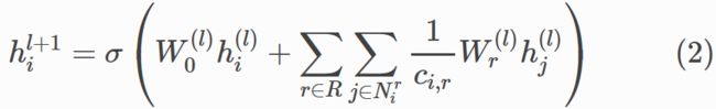
其中 N i r N_i^r Nir表示在满足 r ∈ R r\in R r∈R关系下,节点 i i i的邻居节点集合, c i , r c_i,r ci,r是正则化常数。在实体分类中,R-GCN使用 c i , r = ∣ N i r ∣ c_i,r=| N_i^r| ci,r=∣Nir∣。
直接使用上面的等式存在问题:参数数目增长迅速,尤其对于高度多关系的数据而言。为了减少模型的参数规模和防止过拟合,原始的论文中提出使用基础分解。

因此,权重 W r ( l ) W_r^(l) Wr(l)是基础转换 V b ( l ) V_b^(l) Vb(l)和系数 a r b ( l ) a_rb^(l) arb(l)的线性组合。base的数目 B B B远远小于知识库的关系数目。
DGL中R-GCN的实现
一个R-GCN模型由多个R-GCN层构成。第一个R-GCN层作为输入层,输入与节点实体相关的特征,并映射到隐层空间(如:描述文本)。这里,我们只使用实体ID作为实体特征。
R-GCN层
对于每个节点,一个R-GCN层执行下面的步骤:
- 使用节点表示和与边类型(消息函数)相关的权重矩阵计算输出信息。
- 聚合输入的信息并生成新的节点表示(reduce和apply函数)。
下面定义R-GCN隐藏层的代码。
**!**每种关系类型对应于不同的权重,因此,整个权重矩阵维度为3:关系,输入特征,输出特征。
import torch
import torch.nn.functional as F
from dgl import DGLGraph
import dgl.function as fn
from functools import partial

class RGCNLayer(nn.Module):
	def __init__(self, in_feat, out_feat, num_rels, num_bases=-1, bias=None, activation=None, is_input_layer=False):
		super(RGCNLayer, self).__init__()
		self.in_feat = in_fear
		self.out_feat = out_feat
		self.num_rels = num_rels
		self.num_bases = num_bases
		self.bias =bias
		self.activation = activation
		self.is_input_layer = is_input_layer

		# sanity check(完整性检查)
		if self.num_bases <= 0 or self.num_bases > self.num_rels:
			self.num_bases = self.num_rels

		# weight bases in equation (3)
		self.weight = nn.Parameter(torch.Tensor(self.num_bases, self.in_feat, self.out_feat))

		if self.num_bases < self.num_rels:
		# linear combination coefficients in equation (3)
		self.w_comp = nn.Parameter(torch.Tensor(self.num_rels, self.num_bases))

		# add bias
		if self.bias:
			self.bias = nn.Parameter(torch.Tensor(out_feat))

		# init trainable parameters
		nn.init.xavier_uniform_(self.weight, gain=nn.init.calculate_gain('relu'))

		if self.num_bases < self.num_rels:
			nn.init.xavier_uniform_(self.w_comp, gain=nn.init.calculate_gain('relu'))

		if self.bias:
			nn.init.xavier_uniform_(self.bias, gain=nn.init.calculate_gain('relu'))

	def forward(self, g):
		if self.num_bases < self.num_rels:
			# generate all weights from bases (equation (3))
			weight = self.weight.view(self.in_feat, self.num_bases, self.out_feat)
			weight = torch.matmul(self.w_comp, weight).view(self.num_rels, self.in_feat, self.out_feat)
		else:
			weight = self.weight

		if self.is_input_layer:
			def meaasge_func(edges):
				# for input layer, matrix multiply can be converted to be an embedding lookup using source node id
				embed = weight.view(-1, self.out_feat)
				index = edges.data['rel_type'] * self.in_feat + edges.src['id']
				return {'msg': embed[index] * edges.data['norm']}
		else:
			def message_func(edges):
				w = weight[deges.data['rel_type']]
				msg = torch.bmm(edges.src['h'].unsqueeze(1), w).squeeze()
				msg = msg * edges.data['norm']
				return {'msg': msg}

		def apply_func(nodes):
			h = nodes.data['h']
			if self.bias:
				h = h + self.bias
			if self.activation:
				h = self.activation(h)
			return {'h': h}
		g.update_all(message_func, fn.sum(msg='msg', out='h', apply_func)
完整R-GCN模型定义
class Model(nn.Module):
	def __init__(self, num_nodes, h_dim, out_dim, num_rels, num_bases=-1, num_hidden_layers=1):
		super(Model, self).__init__()
		self.num_nodes = num_nodes
		self.h_dim = h_dim
		self.out_dim = out_dim
		self.num_rels = num_rels
		self.num_bases = num_bases
		self.num_hidden_layers = num_hidden_layers

		# create rgcn layers
		self.features = self.create_features()

	def build_model(self):
		self.layers = nn.ModuleList()
		# input to hidden
		i2h = self.build_input_layer()
		self.layers.append(i2h)
		# hidden to hidden
		for _ in range(self.num_hidden_layers):
			h2h = self.build_hidden_layer()
			self.layers.append(h2h)
		# hidden to output
		h2o = self.build_output_layer()
		self.layers.append(h2o)

	# initialize feature for each node
	def create_features(self):
		features = torch.arange(self.num_nodes)
		return features

	def build_input_layer(self):
		return RGCNLayer(self.num_nodes, self.h_dim, self.num_rels, self.num_bases, activation=F.relu, is_input_layer=True)

	def build_hidden_layer(self):
		return RGCNLayer(self.h_dim, self.h_dim, self.num_rels, self.num_bases, activation=F.relu)

	def build_output_layer(self):
		return RGCNLayer(self.h_dim, self.out_dim, self.num_rels, self.num_bases, activation=partial(F.softmax, dim=1))

	def forward(self, g):
		if self.features is not None:
			g.ndata['id'] = self.features
		for layer in self.layers:
			layer(g)
		return g.ndata.pop('h')
数据集的处理
这里使用R-GCN论文中的应用信息学和形式描述方法研究所(AIFB)数据集。
# load graph data
from dgl.contrib.data import load_data
import numpy as np
data = load_data(dataset='aifb')
num_nodes = data.num_nodes
num_rels = data.num_rels
num_classes = data.num_classes
labels = data.labels
train_idx = data.train_idx
# split training and validation set
val_idx = train_idx[:len(train_idx) // 5]
train_idx = train_idx[len(train_idx) // 5:]

# edge type and normalization factor
edge_type = torch.form_numpy(data.edge_type)
edge_norm = torch.form_numpy(data.edge_norm).unsqueeze(1)

labels = torch.from_numpy(labels).view(-1)
Out:
Loading dataset aifb
Number of nodes:  8285
Number of edges:  66371
Number of relations:  91
Number of classes:  4
removing nodes that are more than 3 hops away
创建图和模型
# configurations
n_hidden = 16 # number of hidden units
n_bases = -1 # use number of relations as number of bases
n_hidden_layers = 0 # use 1 input layer, 1 output layer, no hidden layer
n_epochs = 25 # epochs to train
lr = 0.01 # learning rate
l2norm = 0 # L2 norm coefficient

# create graph
g = DGLGraph()
g.add_nodes(num_nodes)
g.add_edges(data.edge_src, data.edge_dst)
g.edata.update({'rel_type': edge_type, 'norm': edge_norm})

# create model
model = Model(len(g), n_hidden, num_classes, num_rels, num_bases=n_bases, num_hidden_layers=n_hidden_layers)
训练
# optimizer
optimizer = torch.optim.Adam(model.parameters(), lr=lr, weight_decay=l2norm)

print("strat training...")
model.train()
for epoch in range(n_epochs):
	optimizer.zero_grad()
	logits = model.forward(g)
	loss = F.cross_entropy(logits[train_idx], labels[train_idx])
	loss.backward()

	train_acc = torch.sum(logits[train_idx].argmax(dim=1) == labels[train_idx])
	train_acc = train_acc.item() / len(train_idx)
	val_loss = F.cross_entropy(logits[val_idx], labels[val_idx])
	val_acc = torch.sum(logits[val_idx].argmax(dim=1) == labels[val_idx])
	val_acc = val_acc.item() / len(val_idx)
	print("Epoch {:05d} | ".format(epoch) + "Train Accuracy: {:.4f} | Train Loss: {:.4f} | ".format(train_acc, loss.item()) + "Validation Accuracy: {:.4f} | Validation loss: {:.4f}".format(val_acc, val_loss.item()))
Out:
start training...
Epoch 00000 | Train Accuracy: 0.1786 | Train Loss: 1.3866 | Validation Accuracy: 0.1786 | Validation loss: 1.3862
Epoch 00001 | Train Accuracy: 0.9821 | Train Loss: 1.3487 | Validation Accuracy: 0.9643 | Validation loss: 1.3620
Epoch 00002 | Train Accuracy: 0.9821 | Train Loss: 1.2905 | Validation Accuracy: 1.0000 | Validation loss: 1.3259
Epoch 00003 | Train Accuracy: 0.9821 | Train Loss: 1.2137 | Validation Accuracy: 1.0000 | Validation loss: 1.2773
Epoch 00004 | Train Accuracy: 0.9821 | Train Loss: 1.1291 | Validation Accuracy: 1.0000 | Validation loss: 1.2188
Epoch 00005 | Train Accuracy: 0.9821 | Train Loss: 1.0506 | Validation Accuracy: 1.0000 | Validation loss: 1.1536
Epoch 00006 | Train Accuracy: 0.9821 | Train Loss: 0.9850 | Validation Accuracy: 1.0000 | Validation loss: 1.0862
Epoch 00007 | Train Accuracy: 0.9821 | Train Loss: 0.9324 | Validation Accuracy: 1.0000 | Validation loss: 1.0220
Epoch 00008 | Train Accuracy: 0.9821 | Train Loss: 0.8910 | Validation Accuracy: 1.0000 | Validation loss: 0.9659
Epoch 00009 | Train Accuracy: 0.9821 | Train Loss: 0.8588 | Validation Accuracy: 1.0000 | Validation loss: 0.9202
Epoch 00010 | Train Accuracy: 0.9821 | Train Loss: 0.8339 | Validation Accuracy: 1.0000 | Validation loss: 0.8847
Epoch 00011 | Train Accuracy: 0.9821 | Train Loss: 0.8147 | Validation Accuracy: 1.0000 | Validation loss: 0.8571
Epoch 00012 | Train Accuracy: 0.9821 | Train Loss: 0.8001 | Validation Accuracy: 1.0000 | Validation loss: 0.8358
Epoch 00013 | Train Accuracy: 0.9821 | Train Loss: 0.7892 | Validation Accuracy: 1.0000 | Validation loss: 0.8194
Epoch 00014 | Train Accuracy: 0.9821 | Train Loss: 0.7812 | Validation Accuracy: 1.0000 | Validation loss: 0.8071
Epoch 00015 | Train Accuracy: 0.9821 | Train Loss: 0.7752 | Validation Accuracy: 1.0000 | Validation loss: 0.7979
Epoch 00016 | Train Accuracy: 0.9821 | Train Loss: 0.7708 | Validation Accuracy: 0.9643 | Validation loss: 0.7912
Epoch 00017 | Train Accuracy: 0.9821 | Train Loss: 0.7675 | Validation Accuracy: 0.9643 | Validation loss: 0.7864
Epoch 00018 | Train Accuracy: 0.9821 | Train Loss: 0.7650 | Validation Accuracy: 0.9643 | Validation loss: 0.7830
Epoch 00019 | Train Accuracy: 0.9821 | Train Loss: 0.7631 | Validation Accuracy: 0.9643 | Validation loss: 0.7805
Epoch 00020 | Train Accuracy: 0.9821 | Train Loss: 0.7616 | Validation Accuracy: 0.9643 | Validation loss: 0.7787
Epoch 00021 | Train Accuracy: 0.9821 | Train Loss: 0.7603 | Validation Accuracy: 0.9643 | Validation loss: 0.7775
Epoch 00022 | Train Accuracy: 0.9821 | Train Loss: 0.7592 | Validation Accuracy: 0.9643 | Validation loss: 0.7767
Epoch 00023 | Train Accuracy: 0.9821 | Train Loss: 0.7581 | Validation Accuracy: 0.9643 | Validation loss: 0.7762
Epoch 00024 | Train Accuracy: 0.9821 | Train Loss: 0.7570 | Validation Accuracy: 0.9643 | Validation loss: 0.7760
任务二:链路预测
到目前为止,我们已经了解了如何使用DGL通过R-GCN模型实现实体分类。 在知识库设置中,R-GCN生成的表示可用于发现节点之间的潜在关系。 在R-GCN论文中,作者将R-GCN生成的实体表示提供给DistMult预测模型,以预测可能的关系。
该实现与此处介绍的实现类似,但在R-GCN层之上堆叠了一个额外的DistMult层。
代码地址