统计学习方法笔记(七)-线性支持向量机原理及python实现

线性支持向量机

实际场景中训练数据往往不是线性可分的，当训练数据近似线性可分时，就需要使用线性支持向量机或软间隔支持向量机。

给定训练数据集$T=\{(x_1,y_1),(x_2,y_2),...,(x_N,y_N)\}$,其中$\mathcal{X}={\mathcal{R}}^n,y_i\in \mathcal{Y}=\{-1,+1\},i=1,2,...,N$，$x_i$为第$i$个特征向量，$y_i$为$x_i$的类标记.

由于数据中常常有噪声或特异点等，导致数据线性不可分。这就意味着，部分样本点$(x_i,y_i)$不能满足函数间隔大于等于1的约束条件。为此引入松弛变量${\xi }_i$，使得约束条件变为：
$$y_i(w\cdot x_i+b)⩾1-{\xi }_i$$
同时，对每一个松弛变量${\xi }_i$支付一个代价${\xi }_i$.则目标函数变为：
$$\frac{1}{2}\Vert w{\Vert }^2+C\sum _{i=1}^N{\xi }_i$$
其中，$C>0$为惩罚参数.

由此线性不可分的线性支持向量的学习问题转化为凸二次规划问题：
$$\underset{w,b,\xi }{\min }\frac{1}{2}\Vert w{\Vert }^2+C\sum _{i=1}^N{\xi }_i$$
$$s.t{y}_i(w\cdot x_i+b)⩾1-{\xi }_i,i=1,2,...,N$$
$${\xi }_i⩾0,i=1,2,...,N$$

定义 线性支持向量机

对于给定的线性不可分的训练数据集，通过求解凸二次规划问题，即软间隔最大化问题，可得到分离的超平面：$w^{\ast }\cdot x+b^{\ast }$
以及相应的分类决策函数：$f(x)=\mathrm{sign}(w^{\ast }\cdot x+b^{\ast })$，称为线性支持向量机.

线性支持向量机学习算法

输入：训练数据集$T=\{(x_1,y_1),(x_2,y_2),...,(x_N,y_N)\}$,其中$\mathcal{X}={\mathcal{R}}^n,y_i\in \mathcal{Y}=\{-1,+1\},i=1,2,...,N$；

输出：分离超平面和分类决策函数。

第一步:选择惩罚参数$C>0$，构造并求解凸二次规划问题
$$\underset{\alpha }{\min }\frac{1}{2}\sum _{i=1}^N\sum _{j=1}^N{\alpha }_i{\alpha }_j{y}_i{y}_j(x_i\cdot x_j)-\sum _{i=1}^N{\alpha }_i$$

$$s.t.\sum _{i=1}^N{\alpha }_i{y}_i=0$$

$$0⩽{\alpha }_i⩽C,i=1,2,\cdots ,N$$
求得最优化问题的解${\alpha }^{\ast }=({\alpha }_1^{\ast },{\alpha }_2^{\ast },\cdots ,{\alpha }_N^{\ast }{)}^T$

第二步:计算$w^{\ast }={\sum }_{i=1}^N{\alpha }_i^{\ast }{y}_i{x}_i$,并选择${\alpha }^{\ast }$的一个分量$a_j^{\ast }$适合条件$0<{\alpha }_j^{\ast }<C$，计算
$$b^{\ast }=y_i-\sum _{i=1}^N{y}_i{\alpha }_i^{\ast }(x_i\cdot x_j)$$

第三步：求得分离超平面$$w^{\ast }\cdot x+b^{\ast }$$,分类决策函数为:$$f(x)=\mathrm{sign}(w^{\ast }\cdot x+b^{\ast })$$

代码案例 TensorFlow

案例代码已上传：Github地址

import matplotlib.pyplot as plt
import numpy as np
import tensorflow as tf
from sklearn import datasets
from tensorflow.python.framework import ops
ops.reset_default_graph()

# 创建计算图
sess = tf.Session()

第一步：加载数据并划分数据，80%数据用来训练，20%的数据用来做测试

#加载数据
# iris数据 [(Sepal Length, Sepal Width, Petal Length, Petal Width)]
iris = datasets.load_iris()
x_vals = np.array([[x[0], x[3]] for x in iris.data])
y_vals = np.array([1 if y==0 else -1 for y in iris.target])

#加载数据
train_indices = np.random.choice(len(x_vals), round(len(x_vals)*0.8), replace=False)
test_indices = np.array(list(set(range(len(x_vals))) - set(train_indices)))
x_vals_train = x_vals[train_indices]
x_vals_test = x_vals[test_indices]
y_vals_train = y_vals[train_indices]
y_vals_test = y_vals[test_indices]

# 声明参数
batch_size = 100 #批量大小
max_iter=500     #最大迭代次数

# 初始化占位符
x_data = tf.placeholder(shape=[None, 2], dtype=tf.float32)
y_target = tf.placeholder(shape=[None, 1], dtype=tf.float32)

#创建变量
A = tf.Variable(tf.random_normal(shape=[2,1]))
b = tf.Variable(tf.random_normal(shape=[1,1]))


#声明操作 模型
model_output = tf.subtract(tf.matmul(x_data, A), b)

# 声明L2正则化
l2_norm = tf.reduce_sum(tf.square(A))

声明损失函数
$loss=\max (0,1-pred\ast actual)+alpha\ast L{2}_{norm}(A{)}^2$

第二步：声明损失函数并设置优化器、初始化变量

# 声明损失函数
# = max(0, 1-pred*actual) + alpha * L2_norm(A)^2
# L2 正则化参数 alpha
alpha = tf.constant([0.01])
# Margin term in loss
classification_term = tf.reduce_mean(tf.maximum(0., tf.subtract(1., tf.multiply(model_output, y_target))))
# 损失函数
loss = tf.add(classification_term, tf.multiply(alpha, l2_norm))

# 声明预测函数
prediction = tf.sign(model_output)
accuracy = tf.reduce_mean(tf.cast(tf.equal(prediction, y_target), tf.float32))

# 声明优化器
my_opt = tf.train.GradientDescentOptimizer(0.01)
train_step = my_opt.minimize(loss)

# 初始化变量
init = tf.global_variables_initializer()
sess.run(init)

第三步：开始训练

# 开始训练
loss_vec = []
train_accuracy = []
test_accuracy = []
for i in range(max_iter):
    rand_index = np.random.choice(len(x_vals_train), size=batch_size)
    rand_x = x_vals_train[rand_index]
    rand_y = np.transpose([y_vals_train[rand_index]])
    sess.run(train_step, feed_dict={x_data: rand_x, y_target: rand_y})
    
    temp_loss = sess.run(loss, feed_dict={x_data: rand_x, y_target: rand_y})
    loss_vec.append(temp_loss)
    
    train_acc_temp = sess.run(accuracy, feed_dict={x_data: x_vals_train, y_target: np.transpose([y_vals_train])})
    train_accuracy.append(train_acc_temp)
    
    test_acc_temp = sess.run(accuracy, feed_dict={x_data: x_vals_test, y_target: np.transpose([y_vals_test])})
    test_accuracy.append(test_acc_temp)
    
    if (i+1)%100==0:
        print('Step #' + str(i+1) + ' A = ' + str(sess.run(A)) + ' b = ' + str(sess.run(b)))
        print('损失为 ' + str(temp_loss))

# 提取系数
[[a1], [a2]] = sess.run(A)
[[b]] = sess.run(b)
slope = -a2/a1
y_intercept = b/a1

# 提取 x1 and x2 vals
x1_vals = [d[1] for d in x_vals]

# Get best fit line
best_fit = []
for i in x1_vals:
  best_fit.append(slope*i+y_intercept)

# 分离数据
setosa_x = [d[1] for i,d in enumerate(x_vals) if y_vals[i]==1]
setosa_y = [d[0] for i,d in enumerate(x_vals) if y_vals[i]==1]
not_setosa_x = [d[1] for i,d in enumerate(x_vals) if y_vals[i]==-1]
not_setosa_y = [d[0] for i,d in enumerate(x_vals) if y_vals[i]==-1]

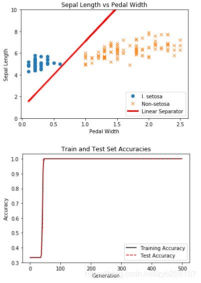
第四步：展示效果

# 分类效果展示
plt.plot(setosa_x, setosa_y, 'o', label='I. setosa')
plt.plot(not_setosa_x, not_setosa_y, 'x', label='Non-setosa')
plt.plot(x1_vals, best_fit, 'r-', label='Linear Separator', linewidth=3)
plt.ylim([0, 10])
plt.legend(loc='lower right')
plt.title('Sepal Length vs Pedal Width')
plt.xlabel('Pedal Width')
plt.ylabel('Sepal Length')
plt.show()

# 训练和测试精度展示
plt.plot(train_accuracy, 'k-', label='Training Accuracy')
plt.plot(test_accuracy, 'r--', label='Test Accuracy')
plt.title('Train and Test Set Accuracies')
plt.xlabel('Generation')
plt.ylabel('Accuracy')
plt.legend(loc='lower right')
plt.show()

案例地址

案例代码已上传：Github地址

参考资料：
[1] 《统计学习方法》
[2]: 《TensorFlow machine learning cookbook》

Github地址https://github.com/Vambooo/lihang-dl

更多技术干货在公众号：深度学习学研社