Mobike数据探索性分析
分析目标
- 获取用户出行的规律,包括时间,日期,路线等
- 对于单车的行驶路径有深入理解
- 对北京运营区域的精细决策
- 为后期建模做准备
变量说明
‘orderid’:订单id
‘userid’:用户id
‘bikeid’:车辆id
‘biketype’:车辆类型
‘starttime’:时间
‘geohashed_start_loc’:骑行出发地(geohash7)
‘geohashed_end_loc’:骑行目的地(geohash7)
‘weekday’:一周中的第几天(周一为0,周日为6)
‘hour’:时间
‘day’:日期
‘start_lat_lng’:出发地纬度和经度
‘end_lat_lng’:目的地纬度和经度
‘start_neighbors’:出发地的相邻8个区域(geohash7)
‘geohashed_start_loc_6’:骑行出发地(geohash6)
‘geohashed_end_loc_6’:骑行目的地(geohash6)
‘start_neighbors_6’:出发地的相邻8个区域(geohash6)
‘geohashed_start_loc_5’:骑行出发地(geohash5)
‘geohashed_end_loc_5’:骑行目的地(geohash5)
‘start_neighbors_5’:出发地的相邻8个区域(geohash5)
‘inside’:目的地是否在出发地以及出发地的相邻区域(geohash7)
‘inside_6’:目的地是否在出发地以及出发地的相邻区域(geohash6)
‘inside_5’:目的地是否在出发地以及出发地的相邻区域(geohash5)
‘start_end_distance’:骑行距离
‘isWeekend’:是否为周末,周末为1,工作日为0
‘geohashed_start_loc_4’:骑行出发地(geohash4)
‘geohashed_end_loc_4’:骑行目的地(geohash4)
‘geohashed_start_loc_3’:骑行出发地(geohash3)
‘geohashed_end_loc_3’:骑行目的地(geohash3)
导入需要的包
# 导入需要的包与库
import pandas as pd
import seaborn as sns
import geohash
import matplotlib.pyplot as plt
from math import radians, cos, sin, asin, sqrt
导入数据
# 导入数据
train = pd.read_csv('C:\\Users\\user\\Desktop\\train.csv',sep = ',',parse_dates = ['starttime'])
观察数据
train.head()
返回结果:

train.shape
返回结果:
![]()
1 数据清洗与整理
def _processData(df):
    # 增加 3列:一周中的哪一天 weekday、小时 hour以及哪一天,并利用时间时期函数从 starttime 中提取
    df['weekday'] = df['starttime'].apply(lambda s : s.weekday()) # Monday is 0 and Sunday is 6
    df['hour'] = df['starttime'].apply(lambda s : s.hour)
    df['day'] = df['starttime'].apply(lambda s : str(s)[:10])

    print("Time process successfully!!!")

    # 将哈希化的地点字符串编码解码为纬度和经度,并且计算出开始骑行地点的 8个相邻区域的经纬度
    df['start_lat_lng'] = df['geohashed_start_loc'].apply(lambda s : geohash.decode(s))
    df['end_lat_lng'] = df['geohashed_end_loc'].apply(lambda s : geohash.decode(s))
    df['start_neighbors'] =  df['geohashed_start_loc'].apply(lambda s : geohash.neighbors(s))

    # 将精度降低,计算哈希化的位置字符串为 6时,开始骑行地点的 8个相邻区域的经纬度
    df['geohashed_start_loc_6'] = df['geohashed_start_loc'].apply(lambda s : s[:6])
    df['geohashed_end_loc_6'] = df['geohashed_end_loc'].apply(lambda s : s[:6])
    df['start_neighbors_6'] =  df['geohashed_start_loc_6'].apply(lambda s : geohash.neighbors(s))

    # 将精度降低,计算哈希化的位置字符串为 5时,开始骑行地点的 8个相邻区域的经纬度
    df['geohashed_start_loc_5'] = df['geohashed_start_loc'].apply(lambda s : s[:5])
    df['geohashed_end_loc_5'] = df['geohashed_end_loc'].apply(lambda s : s[:5])
    df['start_neighbors_5'] =  df['geohashed_start_loc_5'].apply(lambda s : geohash.neighbors(s))

    print("Geohash process successfully!!!")

    # 判断目的地是否在neighbors中
    def inGeohash(start_geohash,end_geohash,names):
        names.append(start_geohash)
        if end_geohash in names:
            return 1
        else:
            return 0
    df['inside'] = df.apply(lambda s :inGeohash(s['geohashed_start_loc'],s['geohashed_end_loc'],s['start_neighbors']),axis = 1)
    df['inside_6'] = df.apply(lambda s :inGeohash(s['geohashed_start_loc_6'],s['geohashed_end_loc_6'],s['start_neighbors_6']),axis = 1)
    df['inside_5'] = df.apply(lambda s :inGeohash(s['geohashed_start_loc_5'],s['geohashed_end_loc_5'],s['start_neighbors_5']),axis = 1)

    print("Geohash inside process successfully!!!")

    # 计算出发地与目的地的距离
    def haversine(lon1, lat1, lon2, lat2):
        """
        Calculate the great circle distance between two points
        on the earth (specified in decimal degrees)
        """
        lon1, lat1, lon2, lat2 = map(radians, [lon1, lat1, lon2, lat2])
        # haversine公式
        dlon = lon2 - lon1
        dlat = lat2 - lat1
        a = sin(dlat/2)**2 + cos(lat1) * cos(lat2) * sin(dlon/2)**2
        c = 2 * asin(sqrt(a))
        r = 6371 # 地球平均半径,单位为公里
        return c * r * 1000
    df["start_end_distance"] = df.apply(lambda s : haversine(s['start_lat_lng'][1],s['start_lat_lng'][0],s['end_lat_lng'][1],s['end_lat_lng'][0]),axis = 1)

    print("Distance process successfully!!!")

    return df
#数据清洗与整理
train = _processData(train)
返回结果:

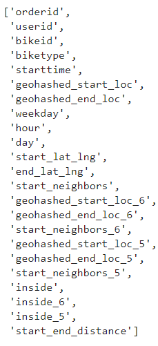
#观察数据集train的列名
train.columns.to_list()
返回结果:
2 时间日期分析
def _timeAnalysis(df):

    # 返回数据集中包含的 Days
    print("数据集包含的天数如下:")
    print(df['day'].unique())
    print('\n',"*"*60,'\n')

    # 用户出行小时高峰期
    print('用户出行小时高峰期:')
    g1 = df.groupby("hour")
    print(g1['orderid'].count().sort_values(ascending =False))
    print('\n',"*"*60,'\n')

    # 周一至周日用车分析
    print('周一至周日用车分析:')
    g1 = df.groupby("weekday")
    print(pd.DataFrame(g1['orderid'].count()))
    print('\n',"*"*60,'\n')

    print('计算工作日与周末每个小时平均的用车量:')
    # 周一至周日不同时间的用车
    df.loc[(df['weekday'] == 5) | (df['weekday'] == 6),"isWeekend"] = 1
    df.loc[~((df['weekday'] == 5) | (df['weekday'] == 6)),"isWeekend"] = 0
    g1 = df.groupby(["isWeekend",'hour'])

    # 计算工作日与周末的天数
    g2 = df.groupby(["day","weekday"])
    w = 0 # 周末天数
    c = 0 # 工作日天数
    for i,j in list(g2.groups.keys()):
        if j >= 5:
            w += 1
        else:
            c +=1

    # 计算工作日与周末每个小时平均的用车量
    temp_df = pd.DataFrame(g1['orderid'].count()).reset_index()
    temp_df.loc[temp_df['isWeekend'] == 0.0,'orderid'] = temp_df['orderid'] / c
    temp_df.loc[temp_df['isWeekend'] == 1.0,'orderid'] = temp_df['orderid'] / w
    print(temp_df.sort_values(["isWeekend","orderid"],ascending =False))
    sns.barplot(x = 'hour',y ="orderid" ,hue = "isWeekend",data = temp_df )
_timeAnalysis(train)
返回结果:


(截取了一部分)

由上述时间分析可知:
- 出行的高峰期为早上7,8点,下午的17,18点;
- 周一到周日的用车量没有明显的区别;
- 工作日中的早晚高峰体现得更明显,周末的用车量相对较平缓。
3 数据可视化与描述性统计
3.1骑行距离分析
# 出行距离的描述统计
train['start_end_distance'].describe()
返回结果:

返回结果表明:75%的用户的骑行距离小于950米,初步说明mobike用户绝大部分为短距离骑行用户
# 绘制出行距离的直方图
from matplotlib import font_manager
my_font = font_manager.FontProperties(fname='C:\\Windows\\Fonts\\times.ttf',size=15)

plt.figure(figsize = (8,6),dpi = 80)
sns.distplot(train['start_end_distance'])
plt.xlabel('start_end_distance',fontproperties=my_font)

plt.show()
返回结果:

受极端值的影响,上图极度右偏,剔除极端值重新观察
# 剔除一些极端的骑行距离案例
start_end_distance = train['start_end_distance']
start_end_distance = start_end_distance.loc[start_end_distance<5000]

plt.figure(figsize = (8,6),dpi = 80)
sns.distplot(start_end_distance)
plt.xlabel('start_end_distance',fontproperties=my_font)

plt.show()
返回结果:

剔除极端影响后,上图可知绝大部分用户骑行距离在2000以内
3.2不同时间对骑行距离的影响
# 不同时间对骑行距离的影响
hour_group = train.groupby("hour")
hour_distance = hour_group.agg({"start_end_distance":"mean"}).reset_index()

plt.figure(figsize = (8,6),dpi = 80)
sns.barplot(x='hour',y='start_end_distance',data=hour_distance)
plt.xlabel('hour',fontproperties=my_font)
plt.ylabel('start_end_distance',fontproperties=my_font)

plt.show()
返回结果:
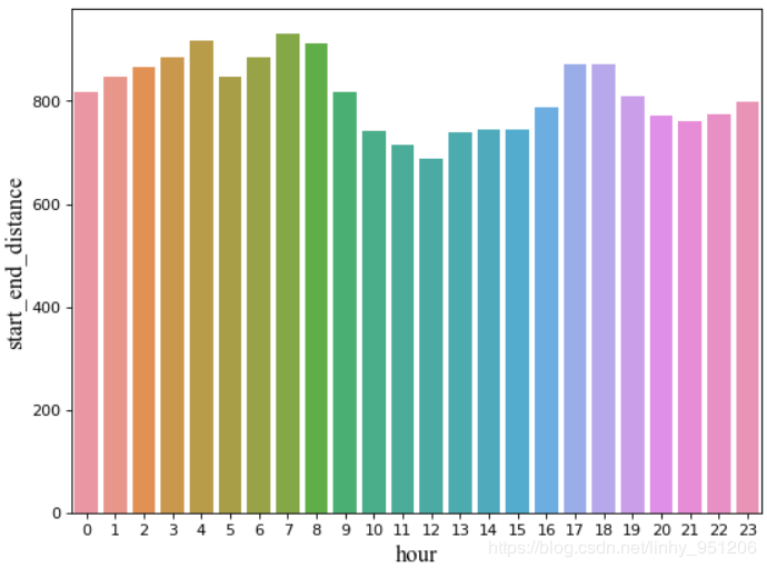
骑行距离不受时间影响
3.3 不同小时出行次数
# 不同小时的出行次数,
hour_group = train.groupby("hour")
hour_num_df = hour_group.agg({"orderid":"count"}).reset_index()

plt.figure(figsize = (8,6),dpi = 80)
sns.barplot(x = "hour",y = "orderid",data =hour_num_df )
plt.xlabel('hour',fontproperties=my_font)
plt.ylabel('orderid_count',fontproperties=my_font)

plt.show()
返回结果:

早晚高峰表现很明显,与实际相符
3.4 工作日与周末不同小时出行次数
# 观察工作日与周末的早晚高峰表现
w_hour_group = train.groupby(["isWeekend","hour"])
w_hour_num_df = w_hour_group.agg({"orderid":"count"}).reset_index()

plt.figure(figsize = (8,6),dpi = 80)
sns.barplot(x = "hour",y = "orderid",data =w_hour_num_df,hue = 'isWeekend')
plt.xlabel('hour',fontproperties=my_font)
plt.ylabel('orderid_count',fontproperties=my_font)

plt.show()
返回结果:

可视化分析得到如下结论:
- mobike用户绝大部分为短距离骑行用户,且75%以上的用户骑行距离在1000米以内;
- 骑行距离在一天中较为平均,不会受时间的影响;
- 在工作日中,上午7、8点,以及下午17、18点是骑行高峰,这与现实中的上下班高峰相对应;
- 工作日中的早晚高峰表现明显,而周末的用车情况相对平缓,且早高峰集中在8到10点。
4 用户出发地与目的地分析
4.1 每天从该点出发或到达的人数/车数
def analysis_1(data,target):
    g1 = data.groupby(['day',target])
    group_data = g1.agg({"orderid":"count","userid":"nunique","bikeid":"nunique"}).reset_index()

    return group_data
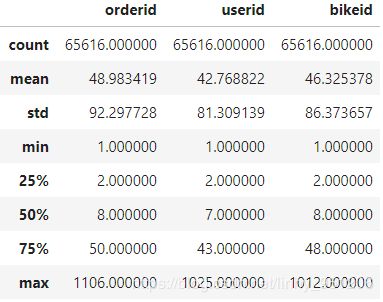
#查看该出发点情况(geohash7)
group_data = analysis_1(train,'geohashed_start_loc')
group_data.describe()
返回结果:

#查看该出发点情况(geohash6)
group_data_6 = analysis_1(train,'geohashed_start_loc_6')
group_data.describe()
返回结果:
#查看该出发点情况(geohash5)
group_data_5 = analysis_1(train,'geohashed_start_loc_5')
group_data.describe()
返回结果:
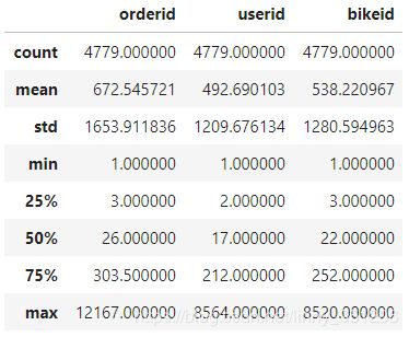
上述分析可知,随着geohash编码位数降低,一天中在某一区域出发的人数/车数都在增加,且一天中,每0.34平方千米(6位编码表示的区域)出发的人数与车数约为45;每10平方千米(5位编码表示的区域)出发到的人数与车数在500左右。
4.2 出发地与目的地组合分析
start_end = train.groupby(["day","geohashed_start_loc","geohashed_end_loc"])

# 计算 出发点-停车点 的 订单量,车辆数,用户数
start_end.agg({"orderid":"count","userid":"nunique","bikeid":"nunique","start_end_distance":"mean"}).reset_index().sort_values(by = "orderid",ascending = False)
返回结果:

(截取一部分)
观察上述结果可知,出发地与目的地的geohash编码前5为往往是相同的
4.3 出发地与目的地之间的关系分析
3.1有关骑行距离的分析中表明,mobike用户绝大部分为短距离骑行用户,
多于75%的用户骑行距离小于1000米,故为探究用户出发点与目的地之间的
关系,应计算各区域的geohash4、geohash3编码(g5和g6的计算在数据
清洗与整理部分)
# 计算g4跟g3
def _geohash(df):

    df['geohashed_start_loc_4'] = df['geohashed_start_loc'].apply(lambda s : s[:4])
    df['geohashed_end_loc_4'] = df['geohashed_end_loc'].apply(lambda s : s[:4])

    df['geohashed_start_loc_3'] = df['geohashed_start_loc'].apply(lambda s : s[:3])
    df['geohashed_end_loc_3'] = df['geohashed_end_loc'].apply(lambda s : s[:3])

    return df
train = _geohash(train)
train.columns.to_list()
返回结果:

# 计算出发点和目的地在不同精度范围内不同的个数
for i in [3,4,5,6]:
    print('g{}'.format(i),':',train.loc[train['geohashed_start_loc_{}'.format(i)] != train['geohashed_end_loc_{}'.format(i)]].shape)
返回结果:

结果显示在g3编码情况下,只有2157条数据的出发地与目的地不同,这与全部数据集条目数(320万)几乎可以忽略不记,则可以说明用户出行地与目的地往往在g3编码下的同一个区域内。
# 计算目的地在出发点g7,g6,g5编码下的neighbors中的个数
for i in ['inside','inside_6','inside_5']:
    print(i,':','\n',train[i].value_counts(),'\n')
返回结果为:

由上述分析可知,在g5编码情况下,出发地与目的地不在同一区域的条目数有75万,而目的地不在出发地的周围8个区域(neighbors)的条目数为7560
用户出发地与目的地分析可以得到如下结论:
- 编码区域越精确(geohash编码位数越长),从某一区域出发的人数与车数越少;
- 在g3编码情况下,用户出发地与目的地往往在同一区域;
- 在g5编码情况下,用户的目的地绝大部分情况下都出现在出发地的附近,这也与前述数据可视化分析中所得出的结论相符:mobike用户为短距离骑行用户。
5 探索分析结论
1、 出行的高峰期为早上7,8点,下午的17,18点;周一到周日的用车量没有明显的区别;工作日中的早晚高峰体现得更明显,周末的用车量相对较平缓。
2、mobike用户绝大部分为短距离骑行用户,且75%以上的用户骑行距离在1000米以内;骑行距离在一天中较为平均,不会受时间的影响;
3、编码区域越精确(geohash编码位数越长),从某一区域出发的人数与车数越少;在g3编码情况下,用户出发地与目的地往往在同一区域;在g5编码情况下,用户的目的地绝大部分情况下都出现在出发地的附近,即表明mobike用户为短距离骑行用户。