【机器学习】吴恩达机器学习视频作业-逻辑回归二分类 II
二分类类型2
本文件的程序是基于吴恩达机器学习视频逻辑回归的作业,使用正则化的逻辑回归,使用的数据是ex2data2.txt。数据背景是:预测来自制造工厂的微芯片是否通过质量保证(QA)。
1 加载数据和数据查看
import numpy as np
import pandas as pd
import matplotlib.pyplot as plt
# 在jupyter整的魔法函数,图形不需要plot即可显示
%matplotlib inline
# 源数据是没有标题的,一行一个样本,每行的前两列是两次成绩,最后一列是是否被录取,每列数据由","隔开,即类似于csv格式数据
# 读取数据到pandas中,并设置列名
pdData = pd.read_csv("ex2data2.txt", header=None, names=['Test1', 'Test2', 'Admitted'])
pdData.head()            # 查看数据的前5行信息
"""
Test1	Test2	Admitted
0	0.051267	0.69956	1
1	-0.092742	0.68494	1
2	-0.213710	0.69225	1
3	-0.375000	0.50219	1
4	-0.513250	0.46564	1
"""
pdData.info()    # 查看数据信息
"""

RangeIndex: 118 entries, 0 to 117
Data columns (total 3 columns):
 #   Column    Non-Null Count  Dtype
---  ------    --------------  -----
 0   Test1     118 non-null    float64
 1   Test2     118 non-null    float64
 2   Admitted  118 non-null    int64
dtypes: float64(2), int64(1)
memory usage: 2.9 KB
"""
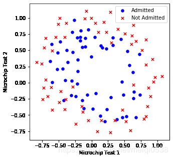
数据可视化
positive = pdData[pdData['Admitted'] == 1]   # 挑选出录取的数据
negative = pdData[pdData['Admitted'] == 0]   # 挑选出未被录取的数据
fig, ax = plt.subplots(figsize=(5, 5))      # 获取绘图对象
# 对录取的数据根据两次考试成绩绘制散点图
ax.scatter(positive['Test1'], positive['Test2'], s=30, c='b', marker='o', label='Admitted')
# 对未被录取的数据根据两次考试成绩绘制散点图
ax.scatter(negative['Test1'], negative['Test2'], s=30, c='r', marker='x', label='Not Admitted')
# 添加图例
ax.legend()
# 设置x,y轴的名称
ax.set_xlabel('Microchip Test 1')
ax.set_ylabel('Microchip Test 2')
## 2 特征映射
从上面的数据可以看出,不能够使用一条直线直接将其划分,我们使用的方法类似于线性回归中多项式线性回归,通过已有的数据创造更多特征(特征映射),这里将多项式达到6次,最后特征数据有(1+2+...+7)28个。
def featureMapping(x1, x2, power):
    # x1: 特征1
    # x2: 特征2
    data = {"f_{}{}".format(i - j, j):
    np.power(x1, i - j)*np.power(x2, j)
    for i in range(power + 1) for j in range(i + 1)
           }
    return pd.DataFrame(data)
x1 = pdData['Test1']
x2 = pdData['Test2']
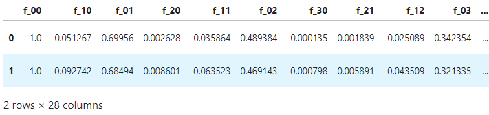
data = featureMapping(x1, x2, 6)
print(data.shape)
"""
(118, 28)
"""
data.head(2)
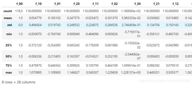
data.describe() # 查看数据描述
3 模型函数
模型函数补办,特征对应的线性函数如下:
Expected node of symbol group type, but got node of type ordgroup
逻辑回归模型函数如下:
h θ ( x ) = g ( θ T x ) h_\theta(x) = g(\theta^T x) hθ(x)=g(θTx)
其中g(z)表达式如下:
g ( z ) = 1 1 + e − z g(z) = \frac{1}{1+e^{-z}} g(z)=1+e−z1
模型使用,我们预测:
当 h θ ( x ) ≥ 0.5 h_\theta(x) \ge 0.5 hθ(x)≥0.5时,预测 y = 1 y=1 y=1
当 h θ ( x ) < 0.5 h_\theta(x) < 0.5 hθ(x)<0.5时,预测 y = 0 y=0 y=0
# 定义一个sigmoid函数
def sigmoid(z):
    # z可以是一个数,也可以是np中的矩阵
    return 1.0/(1+np.exp(-z))
def model(X, theta):
    # 单个数据样本维一个行向量 n个特征, theta为长度为n的行向量
    # 当X为m行n列的数据,返回结果为m行1列的数据
    theta = theta.reshape(1, -1)  # 转成符合矩阵计算
    return sigmoid(X.dot(theta.T))
4 正则化损失函数(Regularize cost)
J ( θ ) = 1 m ∑ i = 1 m [ − y ( i ) log ( h θ ( x ( i ) ) ) − ( 1 − y ( i ) ) log ( 1 − h θ ( x ( i ) ) ) ] + λ 2 m ∑ j = 1 n θ j 2 J(\theta)=\frac{1}{m} \sum_{i=1}^{m}\left[-y^{(i)} \log \left(h_{\theta}\left(x^{(i)}\right)\right)-\left(1-y^{(i)}\right) \log \left(1-h_{\theta}\left(x^{(i)}\right)\right)\right]+\frac{\lambda}{2 m} \sum_{j=1}^{n} \theta_{j}^{2} J(θ)=m1i=1∑m[−y(i)log(hθ(x(i)))−(1−y(i))log(1−hθ(x(i)))]+2mλj=1∑nθj2
特点:比普通的损失函数多了一项 λ 2 m ∑ j = 1 n θ j 2 \frac{\lambda}{2 m} \sum_{j=1}^{n} \theta_{j}^{2} 2mλ∑j=1nθj2,注:此时j从1开始,在之前的损失函数基础上进行改进即可
# 损失函数
def cost(theta, X, y, l=1):
    # X为特征数据集 单个特征数据为行向量形状要为mxn
    # y为标签数据集 为一个列向量形状要为mx1
    # theta为一个行向量 形状要为1xn
    # l 正则化参数,这里默认设置为1
    # 返回一个标量
    left = -y*np.log(model(X, theta))
    right = (1-y)*np.log(1 - model(X, theta))
    return np.sum(left - right)/len(X) + l*np.power(theta[1:], 2).sum()/(2*X.shape[0])
X = np.array(data)               # 已经有常数项了
y = np.array(pdData['Admitted']).reshape(-1, 1)
theta = np.zeros(X.shape[1])
X.shape, y.shape, theta.shape
"""
((118, 28), (118, 1), (28,))
"""
cost(theta, X, y)  #  计算初始损失值
"""
0.6931471805599454
"""
5 计算梯度
正则化梯度公式分为两部分:
∂ J ( θ ) ∂ θ 0 = 1 m ∑ i = 1 m ( h θ ( x ( i ) ) − y ( i ) ) x j ( i ) for j = 1 \frac{\partial J(\theta)}{\partial \theta_{0}}=\frac{1}{m} \sum_{i=1}^{m}\left(h_{\theta}\left(x^{(i)}\right)-y^{(i)}\right) x_{j}^{(i)} \quad \text { for } j = 1 ∂θ0∂J(θ)=m1i=1∑m(hθ(x(i))−y(i))xj(i) for j=1
∂ J ( θ ) ∂ θ j = ( 1 m ∑ i = 1 m ( h θ ( x ( i ) ) − y ( i ) ) x j ( i ) ) + λ m θ j for j ≥ 1 \frac{\partial J(\theta)}{\partial \theta_{j}}=\left(\frac{1}{m} \sum_{i=1}^{m}\left(h_{\theta}\left(x^{(i)}\right)-y^{(i)}\right) x_{j}^{(i)}\right)+\frac{\lambda}{m} \theta_{j} \quad \text { for } j \geq 1 ∂θj∂J(θ)=(m1i=1∑m(hθ(x(i))−y(i))xj(i))+mλθj for j≥1
# 参数的梯度
def gradient(theta, X, y, l=1):
    # X为特征数据集 mxn
    # y为标签数据集 mx1
    # l 正则化参数,默认为1
    # theta为一个行向量 1xn
    grad = ((model(X, theta) - y).T@X).flatten()/ len(X)
    grad[1:] = grad[1:] + l*theta[1:]/X.shape[0]   # 对非常数项参数加上正则项
    # 返回行向量
    return grad
gradient(theta, X, y)   # 查看当前参数下的梯度值
"""
array([8.47457627e-03, 1.87880932e-02, 7.77711864e-05, 5.03446395e-02,
       1.15013308e-02, 3.76648474e-02, 1.83559872e-02, 7.32393391e-03,
       8.19244468e-03, 2.34764889e-02, 3.93486234e-02, 2.23923907e-03,
       1.28600503e-02, 3.09593720e-03, 3.93028171e-02, 1.99707467e-02,
       4.32983232e-03, 3.38643902e-03, 5.83822078e-03, 4.47629067e-03,
       3.10079849e-02, 3.10312442e-02, 1.09740238e-03, 6.31570797e-03,
       4.08503006e-04, 7.26504316e-03, 1.37646175e-03, 3.87936363e-02])
"""
7 使用优化函数计算参数
使用scipy的optimize模块
import scipy.optimize as opt
res = opt.minimize(fun=cost, x0=theta, args=(X,y,1), method='Newton-CG', jac=gradient)
res
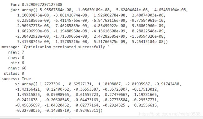
thete_pre = res.x # 获取参数值
8 使用训练得到的参数,计算精确度
# 对数据进行预测
def predict(X, theta):
    # X 训练数据
    # theta 参数
    return [1 if y_pre >= 0.5 else 0 for y_pre in model(X, theta).flatten()]
predictions = predict(X, thete_pre)
correct = [1 if ((a == 1 and b ==1) or (a ==0 and b == 0)) else 0 for (a, b) in zip(predictions, y)]
accuracy = 100*(sum(map(int, correct))/len(correct))       # 计算正确率
# 查看正确率
print('accuracy = {0}%'.format(accuracy))
"""
accuracy = 83.05084745762711%
"""
9 绘制决策边界
也可认为把整个模型封装起来
可以理解为:在数据范围内,如下Test1轴 [-1, 1.5] 和Tes2 [-1, 1.5] 之间找很多点,当点距离曲线 θ T x = 0 \theta^T x = 0 θTx=0很近时,也就是达到一定阈值thresh,就绘制出来,最后就得到了决策边界
# 获取决策边界数据
def getDecisionData(data, density, power, thresh, l):
    # density 样本密度,越大,线条越粗
    t1 = np.linspace(-1, 1.5, density)  # 在-1到1.5之间有density个样本点
    t2 = np.linspace(-1, 1.5, density)
    x_or = np.array(featureMapping(data['Test1'], data['Test2'], power))
    y_or = np.array(data['Admitted']).reshape(-1, 1)
    theta = np.zeros(x_or.shape[1])
    theta = opt.minimize(fun=cost, x0=theta, args=(x_or,y_or, l), method='Newton-CG', jac=gradient).x
    cordinate = [(x, y) for x in t1 for y in t2]  # 构建坐标
    x_cord, y_cord = zip(*cordinate)  # 创造迭代器, *表示拆包
    mapped_cord = featureMapping(x_cord, y_cord, power)
    Y = np.array(mapped_cord) @ theta
    res_data = mapped_cord[np.abs(Y) < thresh]  # 计算的结果 - 0 < thresh 就在曲线指定阈值附近

    # 打印预测结果
    predictions = predict(x_or, theta)
    correct = [1 if ((a == 1 and b ==1) or (a ==0 and b == 0)) else 0 for (a, b) in zip(predictions, y_or)]
    accuracy = 100*(sum(map(int, correct))/len(correct))       # 计算正确率
    # 查看正确率
    print('正则化参数为:{}, 模型正确率为:accuracy = {}%'.format(l,accuracy))

    return res_data.f_10, res_data.f_01   # 获取对应的x,y
def drawDecisionBound(pdData, density, thresh, l):
    x_cor, y_cor = getDecisionData(pdData, density, 6, thresh, l)  # 改变
    positive = pdData[pdData['Admitted'] == 1]   # 挑选出录取的数据
    negative = pdData[pdData['Admitted'] == 0]   # 挑选出未被录取的数据
    fig, ax = plt.subplots(figsize=(5, 5))      # 获取绘图对象
    # 对录取的数据根据两次考试成绩绘制散点图
    ax.scatter(positive['Test1'], positive['Test2'], s=30, c='b', marker='o', label='Admitted')
    # 对未被录取的数据根据两次考试成绩绘制散点图
    ax.scatter(negative['Test1'], negative['Test2'], s=30, c='r', marker='x', label='Not Admitted')
    # 添加图例
    ax.legend()
    # 设置x,y轴的名称
    ax.set_xlabel('Microchip Test 1')
    ax.set_ylabel('Microchip Test 2')
    ax.scatter(x_cor, y_cor, label="fitted curve", s=1)  # s设置点大小
    plt.title("origin data vs fitted curve")
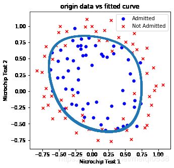
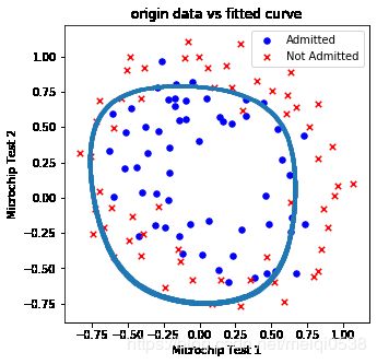
测试1 数据密度为1000,点到决策边界距离阈值0.05,正则项1
drawDecisionBound(pdData, 1000, 0.05, 1)
"""
正则化参数为:1, 模型正确率为:accuracy = 83.05084745762711%
"""
测试2 数据密度为1000,点到决策边界距离阈值0.01,正则项0.8
drawDecisionBound(pdData, 1000, 0.01, 0.8)
"""
正则化参数为:0.8, 模型正确率为:accuracy = 83.05084745762711%
"""
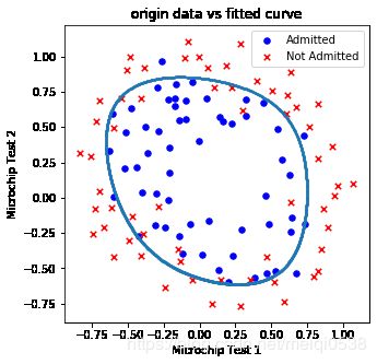
当正则项变化不大的时候正确率没有明显变化(小数据集情况)
测试3 数据密度为1000,点到决策边界距离阈值0.01,正则项0.005
drawDecisionBound(pdData, 1000, 0.01, 0.005)
"""
正则化参数为:0.005, 模型正确率为:accuracy = 83.89830508474576%
"""
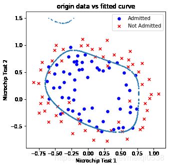
当正则化比较小的时候,解决没有使用正则化处理,那么模型就容易过拟合,测试的正确率就会变大。
测试4 数据密度为1000,点到决策边界距离阈值0.01,正则项0
drawDecisionBound(pdData, 1000, 0.01, 0.)
"""
正则化参数为:0.0, 模型正确率为:accuracy = 87.28813559322035%
"""
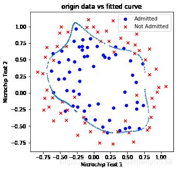
正则项为0,模型过拟合。
测试5 数据密度为1000,点到决策边界距离阈值0.05,正则项1
drawDecisionBound(pdData, 1000, 0.01, 10.)
"""
正则化参数为:10.0, 模型正确率为:accuracy = 74.57627118644068%
"""
当正则项过大时,也会造成欠拟合,正确率底。
总结
上文和本文是使用逻辑回归函数对数据进行二分类,在实际问题中,使用多分类的还是比较多的,下文将介绍如何使用逻辑回归对数据进行多分类。程序源码可在订阅号"AIAS编程有道"中回复“机器学习”即可获取。