python3 Fisher线性判别分析(LDA)(含详细推导和代码)
1、线性判别原理
线性判别分析是常用的降维技术,在模式分类和机器学习的预处理步骤中。其目标是将数据集投影到具有良好的类可分性的低维空间中,以避免过度拟合(维数过多)并降低计算成本,如将一个特征空间(一个数据集n维样本)投射到一个更小的子空间k(其中k ≤n-1)上,同时维护类区分信息。
判别式是一个函数,它接受一个输入向量x,并把它赋值给K个类中的一个,记作![]() 。在这一章中,我们将把注意力限制在线性判别式上,即那些决策面是超平面的判别式。为了简化讨论,我们首先考虑两个类的情况,然后研究K > 2类的扩展。
。在这一章中,我们将把注意力限制在线性判别式上,即那些决策面是超平面的判别式。为了简化讨论,我们首先考虑两个类的情况,然后研究K > 2类的扩展。
1.1 二分类
假设判别面的判别式为: ![]() (因为是线性所以可以直接这么写)
(因为是线性所以可以直接这么写)
若![]() ,则向量x属于类别
,则向量x属于类别 ;若,则向量x属于类别
 。所以决策边界由
 决定。
决定。
假设有两个点 ![]() 和
和  都在决策面上,则
 ![]() ,所以向量 w与决策面上的向量正交且w决定了决策面的方向。
,所以向量 w与决策面上的向量正交且w决定了决策面的方向。
例:假设有三个点![]() 分别在判别面上方,判别面上,判别面下方。则:
分别在判别面上方,判别面上,判别面下方。则:
![]()
![]()
![]()
令![]() , 则
, 则![]() ,因此决策边界的方程式也可以看作原数据点到决策面的距离。
,因此决策边界的方程式也可以看作原数据点到决策面的距离。
原点![]() 到决策面的距离为(用的决策面上的点):
到决策面的距离为(用的决策面上的点):
![]()
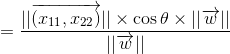

![]()
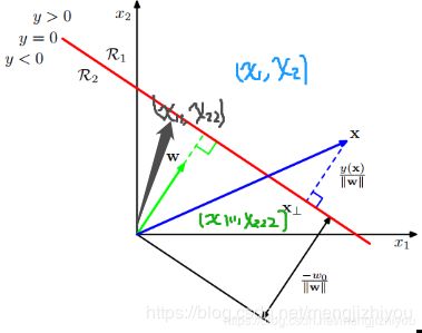
若向量x是决策面外的点,则点到面的距离:
如上图所示,向量x在决策面y=0上的投影点为向量 ,与决策面正交,所以与权重向量w平行,因此向量x可以表示为:
![]()
![]()
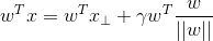
因为 ![]() ,所以:
,所以:
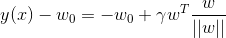
![]()
简化,便于后面计算:
![Y(X)=W^TX(W=[w_0, w],X=[x_0,x])](http://img.e-com-net.com/image/info8/3999dd3a09e4430ea84de54ecca41c09.gif)
注:这里的向量默认的都是列向量,单位法向量是长度为1的法向量=向量/向量的模
1.2 多分类
现在考虑k>2类的情况:
- 一对多(one-versus-the-rest),复杂度K,会导致模糊区域,即数据不属于任何类别
- 一对一(one-versus-one),复杂度K(K - 1)/2,也会导致模糊区域
可以通过考虑一个包含K个线性函数的K类判别器来避免这些问题,则K个类别的判别式形式可以写成:
![]()
如果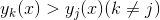 ,则点x属于类别
![]() 。因此类别
。因此类别![]() 和类别
和类别 的决策面是
的决策面是![]() ,所以对于超平面可以定义为:
,所以对于超平面可以定义为:
![]()

上图中, 均属于类别
均属于类别![]() ,则两点连线上的任意点
,则两点连线上的任意点 可以表示为:
![]()
对于线性判别式,则有:

2 、Fisher线性判别分析方法
两个类别:
通过调整权重向量w,找到类分离的最大投影。假设类别有 个点,类别有
 个点,则两个类别的平均向量为:

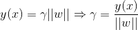
度量类分离最简单的方法是投影类到w上(看下图理解),说明可以选择w来最大化:![]()

左边的图显示了来自两个类的样本(用红色和蓝色表示),以及在连接类的直线上投影得到的直方图。请注意,在投影空间中有相当多的类重叠。右边的图显示了基于Fisher线性判别式的对应投影,显示了极大地改进了类分离。
类别![]() 投影数据的均值可以表示为:
投影数据的均值可以表示为:![]() , 这个表达式可以通过简单地增加w的大小而变得任意大,为此可以让向量w的长度为1,则有
, 这个表达式可以通过简单地增加w的大小而变得任意大,为此可以让向量w的长度为1,则有 。通过引入拉格朗日乘子(拉格朗日乘子)来控制最大化,发现
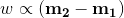 。
。
![]()
![]()
根据上面两个式子以及拉格朗日乘子得到:
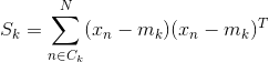
然而,这种方法仍然存在一个问题,如上图所示。这显示了两个类在原始的二维空间(x1, x2)中被很好地分离,但是当它们被投影到连接它们的平均值的直线上时,它们有相当大的重叠。
这种困难来自于类分布的强非对角协方差。Fisher提出的思想是最大化一个函数,该函数将在预计的类均值之间提供一个大的分离,同时在每个类中提供一个小的方差,从而最小化类重叠。
类别![]() 转换后的数据即投影后的数据y的类内方差是:
转换后的数据即投影后的数据y的类内方差是:![]()
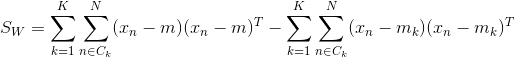
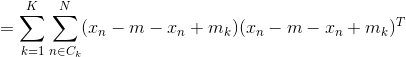
整个数据集的类内协方差可以定义为:![]() , Fisher准则定义类间协方差与类内协方差的比值:
, Fisher准则定义类间协方差与类内协方差的比值:![]()
根据与w的关系,可以写为:
![]()

![]()
![]()
![]()
对 w求导,得:
![]()
![]()
![]()

lambda 是特征值,w是特征向量。另一种理解方式:
![]()
![]() =1
=1
根据拉格朗日乘子:![]() ,其它同上。
,其它同上。
![]() 与
与 同向,此外,因为不考虑w的长度(分子分母均是w的二次项,因此解与w的长度无关),只考虑其方向,所以可以去除伸缩因子
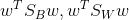 ,然后两边同乘
 ,则有:
,则有:
![]()
多个类别:
考虑 K>2 的类别,假设数据维度D要远大于K。![]() 的计算同上。
的计算同上。

![]()
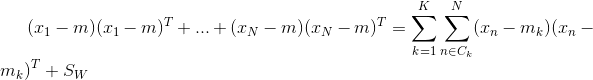
为了找到  的一般形式,为此引入总协方差矩阵(total covariance matrix):


m:所有数据集的平均值,![]() 每个类别的数量,N数据集的总数量,,K是总类别数量,k指某个类别
每个类别的数量,N数据集的总数量,,K是总类别数量,k指某个类别


3、Python3实现
先观察每个特征的分布情况,LDA假设数据是正态分布的,特征是统计独立的,并且每个类都有相同的协方差矩阵。但是,这只适用于LDA作为分类器,如果违背了这些假设,那么降维的LDA也可以很好地工作。
from sklearn import datasets
import matplotlib.pyplot as plt
import numpy as np
import math

# prepare the data
iris = datasets.load_iris()
X = iris.data
y = iris.target
names = iris.feature_names
labels = iris.target_names
y_c = np.unique(y)

"""visualize the distributions of the four different features in 1-dimensional histograms"""
fig, axes = plt.subplots(2, 2, figsize=(12, 6))
for ax, column in zip(axes.ravel(), range(X.shape[1])):
    # set bin sizes
    min_b = math.floor(np.min(X[:, column]))
    max_b = math.ceil(np.max(X[:, column]))
    bins = np.linspace(min_b, max_b, 25)

    # plotting the histograms
    for i, color in zip(y_c, ('blue', 'red', 'green')):
        ax.hist(X[y == i, column], color=color, label='class %s' % labels[i],
                bins=bins, alpha=0.5, )
    ylims = ax.get_ylim()

    # plot annotation
    l = ax.legend(loc='upper right', fancybox=True, fontsize=8)
    l.get_frame().set_alpha(0.5)
    ax.set_ylim([0, max(ylims) + 2])
    ax.set_xlabel(names[column])
    ax.set_title('Iris histogram feature %s' % str(column + 1))

    # hide axis ticks
    ax.tick_params(axis='both', which='both', bottom=False, top=False, left=False, right=False,
                   labelbottom=True, labelleft=True)

    # remove axis spines
    ax.spines['top'].set_visible(False)
    ax.spines["right"].set_visible(False)
    ax.spines["bottom"].set_visible(False)
    ax.spines["left"].set_visible(False)

axes[0][0].set_ylabel('count')
axes[1][0].set_ylabel('count')
fig.tight_layout()
plt.show() 
这些简单的特征图形表示,花瓣的长度和宽度可能更适合分类。
Step 1: Computing the d-dimensional mean vectors
np.set_printoptions(precision=4)

mean_vector = []  # 类别的平均值
for i in y_c:
    mean_vector.append(np.mean(X[y == i], axis=0))
    print('Mean Vector class %s:%s\n' % (i, mean_vector[i]))
Step 2: Computing the Scatter Matrices
"""within-class scatter matrix"""
S_W = np.zeros((X.shape[1], X.shape[1]))
for i in y_c:
    Xi = X[y == i] - mean_vector[i]
    S_W += np.mat(Xi).T * np.mat(Xi)
print('within-class scatter matrix:\n', S_W)

"""between-class scatter matrix """
S_B = np.zeros((X.shape[1], X.shape[1]))
mu = np.mean(X, axis=0)  # 所有样本平均值
for i in y_c:
    Ni = len(X[y == i])
    S_B += Ni * np.mat(mean_vector[i] - mu).T * np.mat(mean_vector[i] - mu)
print('within-class scatter matrix:\n', S_B)
Step 3: Solving the generalized eigenvalue problem for the matrix 
eigvals, eigvecs = np.linalg.eig(np.linalg.inv(S_W) * S_B)  # 求特征值,特征向量
np.testing.assert_array_almost_equal(np.mat(np.linalg.inv(S_W) * S_B) * np.mat(eigvecs[:, 0].reshape(4, 1)),
                                     eigvals[0] * np.mat(eigvecs[:, 0].reshape(4, 1)), decimal=6, err_msg='',
                                     verbose=True)
Step 4: Selecting linear discriminants for the new feature subspace
# sorting the eigenvectors by decreasing eigenvalues
eig_pairs = [(np.abs(eigvals[i]), eigvecs[:, i]) for i in range(len(eigvals))]
eig_pairs = sorted(eig_pairs, key=lambda k: k[0], reverse=True)
W = np.hstack((eig_pairs[0][1].reshape(4, 1), eig_pairs[1][1].reshape(4, 1)))
Step 5: Transforming the samples onto the new subspace
X_trans = X.dot(W)
assert X_trans.shape == (150, 2)
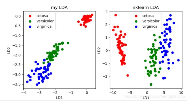
对比sklearn
plt.figure(figsize=(8, 4))
plt.subplot(121)
plt.scatter(X_trans[y == 0, 0], X_trans[y == 0, 1], c='r')
plt.scatter(X_trans[y == 1, 0], X_trans[y == 1, 1], c='g')
plt.scatter(X_trans[y == 2, 0], X_trans[y == 2, 1], c='b')
plt.title('my LDA')
plt.xlabel('LD1')
plt.ylabel('LD2')
plt.legend(labels, loc='best', fancybox=True)

from sklearn.discriminant_analysis import LinearDiscriminantAnalysis

X_trans2 = LinearDiscriminantAnalysis(n_components=2).fit_transform(X, y)
plt.subplot(122)
plt.scatter(X_trans2[y == 0, 0], X_trans2[y == 0, 1], c='r')
plt.scatter(X_trans2[y == 1, 0], X_trans2[y == 1, 1], c='g')
plt.scatter(X_trans2[y == 2, 0], X_trans2[y == 2, 1], c='b')
plt.title('sklearn LDA')
plt.xlabel('LD1')
plt.ylabel('LD2')
plt.legend(labels, loc='best', fancybox=True)