基于OpenCV的（人脸）活性检测

通过本教程，我们将学到如何使用OpenCV进行活体检测。我们将要创建一个活性检测算子。在面部识别系统中发现假的脸（如静止图片）。

过去几年里，我撰写了几篇脸部教程，包括了：

• OpenCV Face Recognition
• Face recognition with dlib, Python, and deep learning
• Raspberry Pi Face Recognition

然而，在邮箱中以及在所发表面部识别文章的评论区中，问得很多次的一个问题是：

 

如何区分真脸和假的脸？

当一个坏人故意破坏你的脸部识别系统，会有发生什么事情。

这样的一个用户会拿着别人的照片。他们可能手举着在手机中的一副照片或者视频，对着脸部识别系统的信息采集摄像头（例如像上面那副图片所示的那样）。

这些情况下，摄像头完全可能对着手机中的图片，识别出一张脸。最终导致一个没授权的用户绕过了你的脸部识别系统。

怎么才可以发现区分开“假的”和“真的、有效的”脸部？怎么把活体检测算法集成到你的面部识别程序中？

答案是：应用本文介绍的基于OpenCV的活体检测算法。

请继续阅读，下文介绍如何把基于OpenCV的活体检测算法集成到面部识别系统中。

本教程的第一部分，我们讨论活体检测，包括了介绍这算法是什么、为什么使用本算法。

我们将要复习一下，为了运用活体检测算法，数据集的一些操作，包括了：

• 怎么建立活体检测的数据集。
• 区分真假面部图片的例子

我们也要说明活体检测算法的工程目录。

为了创建活体检测算子，我们将训练一个能区别真假人脸的深度神经网络

我们因此需要：

1. 练级图片数据集
2. 实现一个能运行活体检测算子的卷积神经网络（我们称之为LivenessNet）
3. 训练活体检测算子网络
4. 创建一个Python+ OpenCV脚本。调用我们训练好的活体检测模型并应用到实时视频中。

让我们开始吧。

什么是活体检测，为什么我们需要活体检测。

图1. 基于OpenCV的活体检测。左边是一段自拍的视频直播（真实的），右边是你们也能看到的我拿着自己的iPhone（假的/伪造的）

脸部识别系统变得越来越流行了，从iPhone或其他智能手机到中国的群众监控。脸部识别系统无处不在。

然而，脸部识别系统容易被一些假的人脸欺骗。

单单地对着识别摄像头举着一张某人的照片（如打印的，手机上的等等），即可绕过脸部识别系统。

为了让脸部识别系统更加安全，我们需要能检测这些假的/非真实的人脸。活体检测就是这种算法的名字。

实现活体检测，有很多种方法，包括了：

3可变聚焦分析(Variable focusing analysis)。评估两个连续帧中的像素变化。
4启发式算法(Heuristic-based algorithms)。包括眼睛动作，嘴唇动作，眨眼检测。这些算法尝试跟踪眼睛的移动以及眨眼，保证用户不是举着别人的照片（因为静止的图片中的人不会眨眼也不会动嘴唇）。

 

There are a number of approaches to liveness detection, including:

• 纹理分析(Texture analysis)。计算面部区域的局部二值模式(Local Binary Patterns)，使用SVM分类真脸和假脸。
• 频率分析(Frequency analysis)。分析脸部的频谱。
• 可变聚焦分析(Variable focusing analysis)。评估两个连续帧中的像素变化。
• 启发式算法(Heuristic-based algorithms)。包括眼睛动作，嘴唇动作，眨眼检测。这些算法尝试跟踪眼睛的移动以及眨眼，保证用户不是举着别人的照片（因为静止的图片中的人不会眨眼也不会动嘴唇）。
• 光流算法。审查3D物体和2D平面的光流特性变化。
• 3D脸部形状。和苹果iPhone脸部识别系统类似，使得系统能区别真脸和打印出来的别人图片。
• 上述的不同组合。使得脸部识别工程师可以选择适合他们应用的检测模型。

活体检测算法的综述可以阅读Chakraborty and Das在2014年的论文：《An Overview of Face liveness Detection》
今天教程的目标是，我们把活体检测看成是一个2进制的分类问题。
对于一张输入照片，我们训练一个能区别真、假人脸的卷积神经网络。
但是在我们训练活体检测模型之前，我们首先考察我们的数据集。

 

我们活体检测视频

图2 手机真脸、假脸样品的例子。左边视频展示的是一个符合规范的我的脸。右边视频展示的是我的手提录的视频
为了让我们的例子直接简洁，我们在本文建立的活体检测算子将致力于区分真脸和屏幕中的假脸。
本算法可以延伸为其他类型的假脸，包括了冲印照片，高像素打印图片等。
为了建立活体检测数据集，我：

 

1. 拿起我的iPhone，打开自拍模式
2. 录制一个25秒的我在办公室走动的视频
3. 重播这段25秒视频，这次将我的iPhone对准我的台式机，让台式机录制视频重播的景象。
4. 这样我们得到了一个真脸的视频，另外一个假脸的视频。
5. 最后，对着两段视频，运用脸部检测，提取出两种分类下的每个脸部的ROIs（就是每张图片都过滤了背景，只留下脸部）。

我提供了真脸、假脸的两段视频文件，请看本文的“下载”部分。

读者可以使用这些视频作为数据集的起点，但是，我建议采集更多的数据，可以帮助建立一个更加鲁棒和精准的活体检测算子。

测试中发现，这模型稍微向我本人的脸偏离。原因是模型训练时用的数据集都是我的。另外，我是白人，我期待同样的数据集适用于不同肤色的人。（译者注：作者是大概是认为自己做实验时候采集到的数据集太小了，图像识别中每个分类达3000个样品很正常）

理想情况下，你在数据集中加入多个人的脸部，同时包括不同的人种。为了改善你的检测模型，请参考“不足点以及将来的工作”提出的建议。

教程的其余部分，你会学习到如何使用OpenCV和深度学习将录制到的数据集转换为实际的活体检测算子。

 

项目结构

直接到“下载”处下载代码、数据集、活体检测模型，解压压缩包。

当你打开工程目录，会发现以下结构：

$ tree --dirsfirst --filelimit 10
.
├── dataset
│   ├── fake [150 entries]
│   └── real [161 entries]
├── face_detector
│   ├── deploy.prototxt
│   └── res10_300x300_ssd_iter_140000.caffemodel
├── pyimagesearch
│   ├── __init__.py
│   └── livenessnet.py
├── videos
│   ├── fake.mp4
│   └── real.mov
├── gather_examples.py
├── train_liveness.py
├── liveness_demo.py
├── le.pickle
├── liveness.model
└── plot.png

6 directories, 12 files

在我们的工程有四个主要文件夹：

• dataset /: 我们的数据集目录包括了两个分类的图片；
  • 当手机播放我的视频时，电脑录制到的手机屏幕而获取得到的假脸，
  • 手机的自拍摄像头捕捉到的我的真脸。
• face_detector/: 包括了我们预训练好的能定位人脸ROIs的Caffe人脸算子。
• pyimagesearch/: 这个模块包括了我们LivenessNet类
• videos/:我提供的给LivenessNet分类器的两个视频输入

现在，我们一起详细分析三段Python代码。到了本文最后，读者们可以往这程序输入个人的数据或者视频。先简单一提，这三段脚本是：

1. gather_examples.py : 这脚本提取了输入视频文件中的脸部ROIs，帮助我们建立一个深度学习人脸活体数据集。
2. train_liveness.py : 正如其名，这段代码将要训练LivenessNet分类器。我们将运用Keras和TensorFLow训练模型。训练结束后会得到一些新文件：
   • le.pickle : 我们的种类标签编码器。
   • liveness.model : 我们序列化的Keras模型。它用于检测人脸活性。
   • plot.png : 这是训练历史的绘图。它展示了精度和损失曲线。我们可以依据它评估我们的模型（过拟合、欠拟合等等。）（译者注：通常是迭代次数不够，称为欠拟合。迭代次数太多，称为过拟合）
3. liveness_demo.py : 我们的演示脚本。这程序会打开webcam，读取各帧图像，实时地执行脸部活体检测。

从我们训练的（视频）数据集检测并提取脸部ROIs

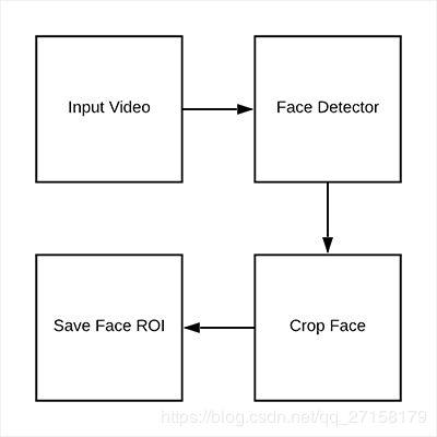
图3. 为了建立活体检测数据集，在视频中检测人脸ROIs

既然我们已经看了我们初始化后的数据集以及工程目录，接下来我们可以通过输入视频，提取真的和假的脸部图像。

这段代码的目标是生成两个文件夹:

1. dataset/fake/: 包含了fake.mp4文件中的脸部ROIs
2. dataset/real/: 包含了real.mov文件中的脸部ROIs

在这样的框架下，我们接下来是用这些图片训练一个基于深度学习的活体检测算子。

打开gather_examples.py文件，插入以下的代码：

# import the necessary packages
import numpy as np
import argparse
import cv2
import os

# construct the argument parse and parse the arguments
ap = argparse.ArgumentParser()
ap.add_argument("-i", "--input", type=str, required=True,
	help="path to input video")
ap.add_argument("-o", "--output", type=str, required=True,
	help="path to output directory of cropped faces")
ap.add_argument("-d", "--detector", type=str, required=True,
	help="path to OpenCV's deep learning face detector")
ap.add_argument("-c", "--confidence", type=float, default=0.5,
	help="minimum probability to filter weak detections")
ap.add_argument("-s", "--skip", type=int, default=16,
	help="# of frames to skip before applying face detection")
args = vars(ap.parse_args())

第2-5行导入我们需要的包。除了内置的Python模块，我们只需要OpenCV和NumPy。

第8-19行解析命令行输入参数：

• --input : 输入视频文件的路径
• --output : 裁剪后的脸部存放的路径
• --detector : 脸部识别算子的路径。我们将要使用OpenCV的深度学习脸部检测算子。这个Caffe模型已经包含在“下载”部分便于大家。
• --confidence : 过滤脸部检测结果的最小可能性阀值。缺省值是50%。
• --skip : 我们不需要处理每一帧图片，因为相邻的数帧图片都是相似的。因此，我们将要跳过N帧进行一次检测。你可以通过命令行改变这个默认值16的参数。

接下来读取脸部检测算子并初始化我们的视频流。

# load our serialized face detector from disk
print("[INFO] loading face detector...")
protoPath = os.path.sep.join([args["detector"], "deploy.prototxt"])
modelPath = os.path.sep.join([args["detector"],
	"res10_300x300_ssd_iter_140000.caffemodel"])
net = cv2.dnn.readNetFromCaffe(protoPath, modelPath)

# open a pointer to the video file stream and initialize the total
# number of frames read and saved thus far
vs = cv2.VideoCapture(args["input"])
read = 0
saved = 0

第23-26行读取OpenCV的深度学习脸部检测算子。

在第30行我们打开视频流。

我们也初始化了两个变量。记录了我们的循环执行中的读取图像数目和保存图像数目。

接下来创建一个循环处理每一帧图像：

# loop over frames from the video file stream
while True:
	# grab the frame from the file
	(grabbed, frame) = vs.read()

	# if the frame was not grabbed, then we have reached the end
	# of the stream
	if not grabbed:
		break

	# increment the total number of frames read thus far
	read += 1

	# check to see if we should process this frame
	if read % args["skip"] != 0:
		continue

我们的while循环在第35行开始：

我们读取并核实一帧图像（第37-42行）

在这个点上，既然我们已经读取了一帧图像，我们将读取计数值递增（第48行）。如果我们跳过一帧特定的图像，我们将跳过本次循环不作任何处理（第48行和第49行）

下一步是检测人脸：

	# grab the frame dimensions and construct a blob from the frame
	(h, w) = frame.shape[:2]
	blob = cv2.dnn.blobFromImage(cv2.resize(frame, (300, 300)), 1.0,
		(300, 300), (104.0, 177.0, 123.0))

	# pass the blob through the network and obtain the detections and
	# predictions
	net.setInput(blob)
	detections = net.forward()

	# ensure at least one face was found
	if len(detections) > 0:
		# we're making the assumption that each image has only ONE
		# face, so find the bounding box with the largest probability
		i = np.argmax(detections[0, 0, :, 2])
		confidence = detections[0, 0, i, 2]

为了运行脸部检测，我们需要创建一个图像的bolb（第53-54行）。为了兼容我们的Caffe脸部检测算子，这个bolb长和高是300x300。之后缩放边框是必需的，因此第52行，获取图像的尺寸。

第58-59行将bolb正向通过深度学习的脸部检测算子。

我们的代码假设视频中每一帧只有一个人脸（第62-65行）。这帮助减少误报。如果你的视频包含了一个以上的人脸，我建议你相应地改变相关逻辑。

因此，第65行获得了脸部检测的最大可能性所在的位置索引。第66行用这个位置索引提取了检测的置信度。

我们过滤掉弱的检测（译者注：置信度较低的检测过滤掉），并将人脸ROI写入硬盘。

		# ensure that the detection with the largest probability also
		# means our minimum probability test (thus helping filter out
		# weak detections)
		if confidence > args["confidence"]:
			# compute the (x, y)-coordinates of the bounding box for
			# the face and extract the face ROI
			box = detections[0, 0, i, 3:7] * np.array([w, h, w, h])
			(startX, startY, endX, endY) = box.astype("int")
			face = frame[startY:endY, startX:endX]

			# write the frame to disk
			p = os.path.sep.join([args["output"],
				"{}.png".format(saved)])
			cv2.imwrite(p, face)
			saved += 1
			print("[INFO] saved {} to disk".format(p))

# do a bit of cleanup
vs.release()
cv2.destroyAllWindows()

第71行保证了检测到的ROI大于阀值，为了降低误报

第74-76行我们提取了脸部ROI的弹框坐标以及脸部ROI本身（第74-76行）。

在第79行-第81行，我们自动为脸部ROI生成了路径+文件名字，并保存到硬盘中。同时，我们所保存到的脸部的数量递增。

一旦处理完成，我们清理了一下，见第86-87行。

建立我们的活体检测图像数据集

 

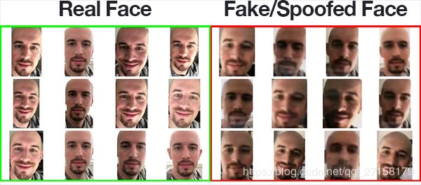
图4 我们OpenCV脸部活体检测数据集。我们将使用Keras和OpenCV训练并演示一个活体模型。

既然我们已经实现了example.py脚本，那么就在工程中调用它。

确保你用本教程的“下载”获取源码和例程、输入视频。

打开终端，执行以下代码提取“假的、伪造”的脸部种类。

$ python gather_examples.py --input videos/fake.mp4 --output dataset/fake \
	--detector face_detector --skip 1
[INFO] loading face detector...
[INFO] saved datasets/fake/0.png to disk
[INFO] saved datasets/fake/1.png to disk
[INFO] saved datasets/fake/2.png to disk
[INFO] saved datasets/fake/3.png to disk
[INFO] saved datasets/fake/4.png to disk
[INFO] saved datasets/fake/5.png to disk
...
[INFO] saved datasets/fake/145.png to disk
[INFO] saved datasets/fake/146.png to disk
[INFO] saved datasets/fake/147.png to disk
[INFO] saved datasets/fake/148.png to disk
[INFO] saved datasets/fake/149.png to disk

同样的，我们对“真实的”种类也进行同样的操作：

$ python gather_examples.py --input videos/real.mov --output dataset/real \
	--detector face_detector --skip 4
[INFO] loading face detector...
[INFO] saved datasets/real/0.png to disk
[INFO] saved datasets/real/1.png to disk
[INFO] saved datasets/real/2.png to disk
[INFO] saved datasets/real/3.png to disk
[INFO] saved datasets/real/4.png to disk
...
[INFO] saved datasets/real/156.png to disk
[INFO] saved datasets/real/157.png to disk
[INFO] saved datasets/real/158.png to disk
[INFO] saved datasets/real/159.png to disk
[INFO] saved datasets/real/160.png to disk

由于“真实的”视频文件长于“伪造的”视频文件，我们将跳过更多的帧数以平衡两个种类的输出脸部ROIs数量。

执行代码以后，得到了以下的图像数目：

• 伪造的：150幅图像
• 真实的：161幅图像
• 总计：311幅图像。

实现深度学习活体检测算子“LivenessNet”

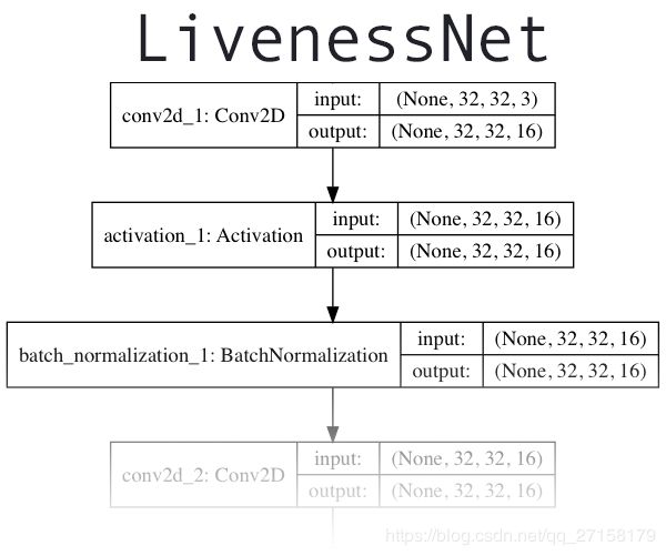
图5 LivenessNet的深度学习框架是一个用于检测图像和视频中的脸部活体卷积神经网络

下一步实现了我们的深度学习活体检测算子“LivenessNet”

本质上，LivenessNet只是一个简单的卷积神经网络

我们故意将网络的结构保持简单，并保持尽量少的参数。这样的原因有两个：

1. 减少在小数据集中过拟合的机会
2. 保证我们的活体检测算子是快速的，可以实时运行（即使在资源有限的设备中如树莓派）

接下来运行LivenessNet。创建livenessnet.py并输入以下代码：

# import the necessary packages
from keras.models import Sequential
from keras.layers.normalization import BatchNormalization
from keras.layers.convolutional import Conv2D
from keras.layers.convolutional import MaxPooling2D
from keras.layers.core import Activation
from keras.layers.core import Flatten
from keras.layers.core import Dropout
from keras.layers.core import Dense
from keras import backend as K

class LivenessNet:
	@staticmethod
	def build(width, height, depth, classes):
		# initialize the model along with the input shape to be
		# "channels last" and the channels dimension itself
		model = Sequential()
		inputShape = (height, width, depth)
		chanDim = -1

		# if we are using "channels first", update the input shape
		# and channels dimension
		if K.image_data_format() == "channels_first":
			inputShape = (depth, height, width)
			chanDim = 1

All of our imports are from Keras (Lines 2-10). For an in-depth review of each of these layers and functions, be sure to refer to Deep Learning for Computer Vision with Python.

全部导入的模块都输入Keras（第2-10行）。如果想深度分析每一层的代码以及作用，请参考Deep Learning for Computer Vision with Python。

我们的LivenessNet种类定义在第12行。它包括了一个静态函数build()（见第14行）。build()函数接受4种参数：

• 宽度width ：图像的宽度
• 高度height ：图像的高度.
• 深度depth ：图像的通道数（本场合由于是RGB图像，有3个通道）
• 种类classes：种类的数目。在这里我们有两个种类：“真实的”和“伪造的”

第17行初始化了我们的模型。

第18行定义了我们模型的输入形状。第23

接下来，增加我们CNN卷积神经网络的层数：

		# first CONV => RELU => CONV => RELU => POOL layer set
		model.add(Conv2D(16, (3, 3), padding="same",
			input_shape=inputShape))
		model.add(Activation("relu"))
		model.add(BatchNormalization(axis=chanDim))
		model.add(Conv2D(16, (3, 3), padding="same"))
		model.add(Activation("relu"))
		model.add(BatchNormalization(axis=chanDim))
		model.add(MaxPooling2D(pool_size=(2, 2)))
		model.add(Dropout(0.25))

		# second CONV => RELU => CONV => RELU => POOL layer set
		model.add(Conv2D(32, (3, 3), padding="same"))
		model.add(Activation("relu"))
		model.add(BatchNormalization(axis=chanDim))
		model.add(Conv2D(32, (3, 3), padding="same"))
		model.add(Activation("relu"))
		model.add(BatchNormalization(axis=chanDim))
		model.add(MaxPooling2D(pool_size=(2, 2)))
		model.add(Dropout(0.25))

我们的CNN展示了 VGGNet-esque的品质。它很浅，带有一些少量的学习过滤器。事实上，我们不需要一个很深的网络区别真的和假的脸部。

第一个 CONV => RELU => CONV => RELU => POOL层组在第28-36行指定了。同时增加了批标准化(BN)和dropout层。

第39-46增加了另一个CONV => RELU => CONV => RELU => POOL层组。

网络的尾部是我们的FC=>RELU层:

		# first (and only) set of FC => RELU layers
		model.add(Flatten())
		model.add(Dense(64))
		model.add(Activation("relu"))
		model.add(BatchNormalization())
		model.add(Dropout(0.5))

		# softmax classifier
		model.add(Dense(classes))
		model.add(Activation("softmax"))

		# return the constructed network architecture
		return model

第49-57行，表示了输出层是全连接的用ReLU激活的，并使用softmax分类器。

第60行，return模型到训练程序。

创建活体检测算子训练脚本：

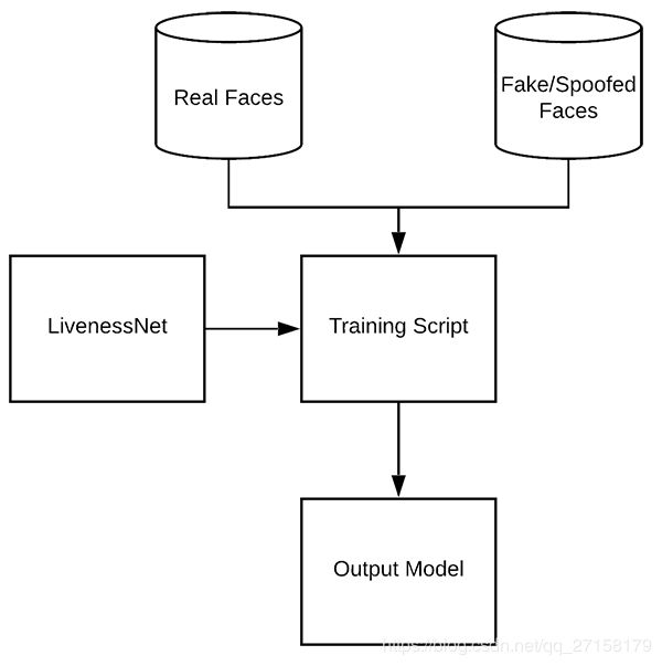
图6 训练LivenessNet的过程。采用我们数据集中的“真实的”和“伪造的”图像，使用OpenCV、Keras和深度学习训练活体检测模型。

数据集和LivenessNet都初始化后，我们可以训练网络了。

创建train_liveness.py文件，输入以下代码：

# set the matplotlib backend so figures can be saved in the background
import matplotlib
matplotlib.use("Agg")

# import the necessary packages
from pyimagesearch.livenessnet import LivenessNet
from sklearn.preprocessing import LabelEncoder
from sklearn.model_selection import train_test_split
from sklearn.metrics import classification_report
from keras.preprocessing.image import ImageDataGenerator
from keras.optimizers import Adam
from keras.utils import np_utils
from imutils import paths
import matplotlib.pyplot as plt
import numpy as np
import argparse
import pickle
import cv2
import os

# construct the argument parser and parse the arguments
ap = argparse.ArgumentParser()
ap.add_argument("-d", "--dataset", required=True,
	help="path to input dataset")
ap.add_argument("-m", "--model", type=str, required=True,
	help="path to trained model")
ap.add_argument("-l", "--le", type=str, required=True,
	help="path to label encoder")
ap.add_argument("-p", "--plot", type=str, default="plot.png",
	help="path to output loss/accuracy plot")
args = vars(ap.parse_args())

我们脸部活性训练模型包括了一些导入（见第2-19行）

• matplotlib : 用于生成训练情况绘图。我们指定Agg后端，便于将绘图保存到硬盘。见第3行。
• LivenessNet : 之前提到的我们定义好了活体CNN网络。
• train_test_split :scikit-learn的一个函数，用于分离训练和测试的样品
• classification_report :来自scikit-learn中。生成模型运行表现的简要统计报告。
• ImageDataGenerator :用于数据扩充。让我们可以随机地变异现有图像（译者注：增大数据集容量）。
• Adam : 模型的优化器。（也可以选择SGD，RMSprop等）
• paths : imutils的模块。帮我们获取硬盘中图像文件的路径。
• pyplot :用于生成一个好看的训练绘图。
• numpy : 一个Python数字处理库。也是OpenCV的运行需要的。
• argparse :用于解析命令行参数
• pickle : 用于将标签编译器保存到硬盘。
• cv2 : 我们的OpenCV。
• os : 这模块有很多作用。但我们只用于分离操作系统路径。

这真是啰嗦。不过如果知道上面导入的内容，那么下面审查代码就变得很简单了。

本代码支持四个参数输入。

• --dataset : 输入数据集的路径。本文已经提到用gather_example.py创建数据集。
• --model : 我们的代码将要生成输出模型文件，在这里要提供路径。
• --le : 我们输出标签编码器的路径也是需要提供的。
• --plot : 训练程序会生成一个绘图。如果你想覆盖缺省值“plot.png”，你可以在命令行中指定这个参数。

下一段代码将要执行一系列的初始化，并创建我们的数据。

# initialize the initial learning rate, batch size, and number of
# epochs to train for
INIT_LR = 1e-4
BS = 8
EPOCHS = 50

# grab the list of images in our dataset directory, then initialize
# the list of data (i.e., images) and class images
print("[INFO] loading images...")
imagePaths = list(paths.list_images(args["dataset"]))
data = []
labels = []

for imagePath in imagePaths:
	# extract the class label from the filename, load the image and
	# resize it to be a fixed 32x32 pixels, ignoring aspect ratio
	label = imagePath.split(os.path.sep)[-2]
	image = cv2.imread(imagePath)
	image = cv2.resize(image, (32, 32))

	# update the data and labels lists, respectively
	data.append(image)
	labels.append(label)

# convert the data into a NumPy array, then preprocess it by scaling
# all pixel intensities to the range [0, 1]
data = np.array(data, dtype="float") / 255.0

训练参数包括了初始的学习速度，批尺寸（batch size）和迭代次数，见第35-37行。

第42-44行，我们获得了imagePaths。我们初始化了两个列表，存放我们的数据和种类标签。

第46-55行代码的循环，建立了我们的数据和标签列表。数据是我们读取并将尺寸改为32x32。每一张图片都有对应的标签存放在labels列表。

每一个像素的密集度用[0,1]表示。第59行用NumPy数组创建这个列表。

编码我们的标签以及划分我们的数据。

# encode the labels (which are currently strings) as integers and then
# one-hot encode them
le = LabelEncoder()
labels = le.fit_transform(labels)
labels = np_utils.to_categorical(labels, 2)

# partition the data into training and testing splits using 75% of
# the data for training and the remaining 25% for testing
(trainX, testX, trainY, testY) = train_test_split(data, labels,
	test_size=0.25, random_state=42)

第63-65行将标签进行编码。

我们使用scikit-learn分类数据。75%用于训练，25%用于测试，见第69-70行。

初始化我们的数据扩充目标，并编译+训练我们的脸部活体模型：

# construct the training image generator for data augmentation
aug = ImageDataGenerator(rotation_range=20, zoom_range=0.15,
	width_shift_range=0.2, height_shift_range=0.2, shear_range=0.15,
	horizontal_flip=True, fill_mode="nearest")

# initialize the optimizer and model
print("[INFO] compiling model...")
opt = Adam(lr=INIT_LR, decay=INIT_LR / EPOCHS)
model = LivenessNet.build(width=32, height=32, depth=3,
	classes=len(le.classes_))
model.compile(loss="binary_crossentropy", optimizer=opt,
	metrics=["accuracy"])

# train the network
print("[INFO] training network for {} epochs...".format(EPOCHS))
H = model.fit_generator(aug.flow(trainX, trainY, batch_size=BS),
	validation_data=(testX, testY), steps_per_epoch=len(trainX) // BS,
	epochs=EPOCHS)

第73-75构建了数据扩充目标，生成了随机的旋转，缩放，漂移，裁剪，翻转。想知道更多的数据扩充，请看 my previous blog post。

我们LivenessNet模型建立以及编译，在第79-83行。

第87-89行我们开始训练。对于我们这么浅的网络以及小型数据集，这个过程是相对快速的。

一旦模型训练好，我们可以评估结果，并生成一个训练绘图：

# evaluate the network
print("[INFO] evaluating network...")
predictions = model.predict(testX, batch_size=BS)
print(classification_report(testY.argmax(axis=1),
	predictions.argmax(axis=1), target_names=le.classes_))

# save the network to disk
print("[INFO] serializing network to '{}'...".format(args["model"]))
model.save(args["model"])

# save the label encoder to disk
f = open(args["le"], "wb")
f.write(pickle.dumps(le))
f.close()

# plot the training loss and accuracy
plt.style.use("ggplot")
plt.figure()
plt.plot(np.arange(0, EPOCHS), H.history["loss"], label="train_loss")
plt.plot(np.arange(0, EPOCHS), H.history["val_loss"], label="val_loss")
plt.plot(np.arange(0, EPOCHS), H.history["acc"], label="train_acc")
plt.plot(np.arange(0, EPOCHS), H.history["val_acc"], label="val_acc")
plt.title("Training Loss and Accuracy on Dataset")
plt.xlabel("Epoch #")
plt.ylabel("Loss/Accuracy")
plt.legend(loc="lower left")
plt.savefig(args["plot"])

第93行，对测试数据进行预测。随后生成了一个分类报告，并在终端打印（第94-95行）

第99-104行，LivenessNet模型和标签的编码器一同保存到硬盘。

剩余的第107-117行生成一个训练历史绘图，以后可以查看。

训练我们的活体检测算子

我们现在已经准备好可以训练我们的活体训练算子了。

确保你的代码和数据集是从本教程“下载”部分得到的。执行以下代码：

$ python train.py --dataset dataset --model liveness.model --le le.pickle
[INFO] loading images...
[INFO] compiling model...
[INFO] training network for 50 epochs...
Epoch 1/50
29/29 [==============================] - 2s 58ms/step - loss: 1.0113 - acc: 0.5862 - val_loss: 0.4749 - val_acc: 0.7436
Epoch 2/50
29/29 [==============================] - 1s 21ms/step - loss: 0.9418 - acc: 0.6127 - val_loss: 0.4436 - val_acc: 0.7949
Epoch 3/50
29/29 [==============================] - 1s 21ms/step - loss: 0.8926 - acc: 0.6472 - val_loss: 0.3837 - val_acc: 0.8077
...
Epoch 48/50
29/29 [==============================] - 1s 21ms/step - loss: 0.2796 - acc: 0.9094 - val_loss: 0.0299 - val_acc: 1.0000
Epoch 49/50
29/29 [==============================] - 1s 21ms/step - loss: 0.3733 - acc: 0.8792 - val_loss: 0.0346 - val_acc: 0.9872
Epoch 50/50
29/29 [==============================] - 1s 21ms/step - loss: 0.2660 - acc: 0.9008 - val_loss: 0.0322 - val_acc: 0.9872
[INFO] evaluating network...
              precision    recall  f1-score   support

        fake       0.97      1.00      0.99        35
        real       1.00      0.98      0.99        43

   micro avg       0.99      0.99      0.99        78
   macro avg       0.99      0.99      0.99        78
weighted avg       0.99      0.99      0.99        78

[INFO] serializing network to 'liveness.model'...

图6. 用OpenCV、Keras和深度学习训练脸部活体模型并画图

结果显示，对于我们的验证数据，可以得到99%的活体检测精度。

综合以上的各部分：基于OpenCV的活体检测算法

综合以上的各部分：基于OpenCV的活体检测算法

图7 用OpenCV和深度学习的脸部活体检测

最后一步结合所有的部分：

1. 我们读取webcam/视频流
2. 对每帧图像应用脸部检测
3. 对于每个脸部，应用我们的活体检测模型

打开liveness_demo.py，并插入以下代码：

# import the necessary packages
from imutils.video import VideoStream
from keras.preprocessing.image import img_to_array
from keras.models import load_model
import numpy as np
import argparse
import imutils
import pickle
import time
import cv2
import os

# construct the argument parse and parse the arguments
ap = argparse.ArgumentParser()
ap.add_argument("-m", "--model", type=str, required=True,
	help="path to trained model")
ap.add_argument("-l", "--le", type=str, required=True,
	help="path to label encoder")
ap.add_argument("-d", "--detector", type=str, required=True,
	help="path to OpenCV's deep learning face detector")
ap.add_argument("-c", "--confidence", type=float, default=0.5,
	help="minimum probability to filter weak detections")
args = vars(ap.parse_args())

第2-11行导入我们所需要的模块。我们使用：

• VideoStream  读取我们的摄像头
• img_to_array  我们的每帧图像都要转换到一个兼容的数组格式
• load_model  读取我们的序列化Keras模型
• imutils   提供了些方便的功能。
• cv2  OPenCV

第14-23行解析我们命令行形参：

• --model : 用于活体检测的我们提前训练好的Keras模型的路径
• --le :标签编码器的路径
• --detector : OpenCV的深度学习脸部识别器的路径，用于找到脸部ROIs
• --confidence : 过滤掉弱检测的最小可能性阀值

接下来，初始化一个脸部识别器，LivenessNet模型和标签编码器，和视频流。

# load our serialized face detector from disk
print("[INFO] loading face detector...")
protoPath = os.path.sep.join([args["detector"], "deploy.prototxt"])
modelPath = os.path.sep.join([args["detector"],
	"res10_300x300_ssd_iter_140000.caffemodel"])
net = cv2.dnn.readNetFromCaffe(protoPath, modelPath)

# load the liveness detector model and label encoder from disk
print("[INFO] loading liveness detector...")
model = load_model(args["model"])
le = pickle.loads(open(args["le"], "rb").read())

# initialize the video stream and allow the camera sensor to warmup
print("[INFO] starting video stream...")
vs = VideoStream(src=0).start()
time.sleep(2.0)

第27-30行读取了OpenCV脸部识别算子。

第34-35行，我们读取了序列化、预训练好的模型（LivenessNet）和标签编码器。

第39-40行我们的视频流对象实例化。摄像头有两秒开机热机时间。

是时候开始循环处理每一帧图像，检测真、假脸部。

# loop over the frames from the video stream
while True:
	# grab the frame from the threaded video stream and resize it
	# to have a maximum width of 600 pixels
	frame = vs.read()
	frame = imutils.resize(frame, width=600)

	# grab the frame dimensions and convert it to a blob
	(h, w) = frame.shape[:2]
	blob = cv2.dnn.blobFromImage(cv2.resize(frame, (300, 300)), 1.0,
		(300, 300), (104.0, 177.0, 123.0))

	# pass the blob through the network and obtain the detections and
	# predictions
	net.setInput(blob)
	detections = net.forward()

第43行是一个死循环，里面读取并改变了每一帧的尺寸（第46-47行）。

随后，每一帧的尺寸都被读取，之后进行缩放（第50行）

使用OpenCV自带的blobFromImage函数，我们生成一个blob（第51-52行）。然后将其输入到脸部识别网络，做推断（第56-57行）。

我们到了有趣的部分——使用OpenCV和深度学习的活体检测。

	# loop over the detections
	for i in range(0, detections.shape[2]):
		# extract the confidence (i.e., probability) associated with the
		# prediction
		confidence = detections[0, 0, i, 2]

		# filter out weak detections
		if confidence > args["confidence"]:
			# compute the (x, y)-coordinates of the bounding box for
			# the face and extract the face ROI
			box = detections[0, 0, i, 3:7] * np.array([w, h, w, h])
			(startX, startY, endX, endY) = box.astype("int")

			# ensure the detected bounding box does fall outside the
			# dimensions of the frame
			startX = max(0, startX)
			startY = max(0, startY)
			endX = min(w, endX)
			endY = min(h, endY)

			# extract the face ROI and then preproces it in the exact
			# same manner as our training data
			face = frame[startY:endY, startX:endX]
			face = cv2.resize(face, (32, 32))
			face = face.astype("float") / 255.0
			face = img_to_array(face)
			face = np.expand_dims(face, axis=0)

			# pass the face ROI through the trained liveness detector
			# model to determine if the face is "real" or "fake"
			preds = model.predict(face)[0]
			j = np.argmax(preds)
			label = le.classes_[j]

			# draw the label and bounding box on the frame
			label = "{}: {:.4f}".format(label, preds[j])
			cv2.putText(frame, label, (startX, startY - 10),
				cv2.FONT_HERSHEY_SIMPLEX, 0.5, (0, 0, 255), 2)
			cv2.rectangle(frame, (startX, startY), (endX, endY),
				(0, 0, 255), 2)

 

第60行，我们开始循环执行脸部检测。在这里，我们：

• 过滤掉弱检测（第63-66行）
• 提取脸部弹框的坐标，并保存不会坐落到图像的边缘之外（第69-77行）。
• 提取脸部ROI，然后用处理训练数据的方法进行预处理。
• 使用我们的活体检测模型判断脸部是真实的还是伪造的。
• 第91行，你会插入你的代码，只对真实的图像进行脸部识别。这段程度的伪代码类似于 if label == "real": run_face_reconition()
• 本次demo的最终，我们画出标签文字和矩阵框，以标记出脸部（第94-98行）

显示结果，并做下清理。

	# show the output frame and wait for a key press
	cv2.imshow("Frame", frame)
	key = cv2.waitKey(1) & 0xFF

	# if the `q` key was pressed, break from the loop
	if key == ord("q"):
		break

# do a bit of cleanup
cv2.destroyAllWindows()
vs.stop()

每次的循环，当检测到键盘按键后，输出图像（第101-102行）。每当用户按下“q”，我们会跳出循环，释放 指针，关闭窗口（第105-110行）

对实时视频部署我们的活体检测算子

如果是要跟着我们的demo跑，请确保是从本文的“下载”部分获取到的代码、预训练好的活体检测模型。

打开终端并执行以下代码：

$ python liveness_demo.py --model liveness.model --le le.pickle \
	--detector face_detector
Using TensorFlow backend.
[INFO] loading face detector...
[INFO] loading liveness detector...
[INFO] starting video stream...

这样，可以看到我们活体检测算子可以成功区分真实的伪造的人脸。

我将在下面的视频中，展示一个更长的demo。

不足点，改善之处以及将来的工作

不足点，改善之处以及将来的工作

我们活体检测算子最首要局限在于我们受限的数据集，只有总数为311张。（161是真实的种类，150是伪造的种类）。

本工作的一个工作延伸是简单的收集额外的训练数据，更详细的是，图像不能仅仅是你和我。

要记得本例子数据集只包括了一个人的脸部。同样作者本身是白人，你可以手机更多的训练脸部或者其他肤色的人种。

我们的活体检测算子的训练集中，伪造的样品都是手机屏幕中的。并没有使用打印出来的图片进行训练。因此，我的第三个建议是，不要只录制手机屏幕，而是采取更多的方式获得伪造人脸图像。

最后，我想提醒大家，活体检测算法并没有银色子弹（译者注：意思是没有完美的一种活体检测算法）

一些最好的活体检测算子继承了多个活体检测方法（请参考前文的“什么是活体检测，为什么要活体检测”）

挤出时间，考虑并评估一下项目、指引、需求。某些情况下，你所需要的可能仅仅是基本的眨眼检测。

另外的情况下，你可能需要结合深度学习检测和其他试探法，

不要盲目冲进脸部识别和活体检测，花时间想想，别冲动，想想你自身独特的项目需求。这样能保证你会获得更好更准确的结果。

总结

本教程，学会了如何用OpenCV执行活体检测

使用这个活体检测算子，可以发现伪造的脸部，同时在自己的脸部识别系统中排除掉尝试用脸部欺骗的人脸验证。

使用OpenCV深度学习，Python创建了活体检测算子

第一步是采集我们的真的vs假的数据集。为了完成这个任务，我们：

1. 首先用智能手机自拍模式录制了我们的视频
2. 将我们的手机对着笔记本、台式机，重播上面的视频，使用我们的webcam录制并回放视频。
3. 对两段视频，采用脸部识别，构造我们的活体检测数据集

建立好数据集，我们实现了“LivenessNet”，一个Keras+深度学习的CNN网络。

这个网络故意做得浅，保证了：

1. 在我们的小型数据集中，减少了过拟合的机会
2. 模型本身可以实时运行（树莓派也可以）

总的来说，我们活体检测算子在我们的验证组中能获取99%的精度。

为了演示这个活体检测通道，我们创建了Python+OpenCV脚本，读取了我们活体检测算子并应用到实时视频流当中。

像我们demo展示的那样，我们的活体检测算子能区别出真的和伪造的人脸。

我希望你们能享受今天我就基于OpenCV实现活体检测的文章。

 

 

原文链接：https://www.pyimagesearch.com/2019/03/11/liveness-detection-with-opencv/

免责声明：请大家支持原创，本文是翻译的。只作学习用途。文中所有图片均来自pyimagesearch。若侵权，请联系我。我的QQ是77028629。