小呆学数据分析——House Prices房价预测
文章目录
- 0. 问题
- 1.数据分析
- 1.1 初识数据
- 1.2 缺失值分析和处理
- None
- 0 值
- Miss
- 处理缺失值
- 1.3 数值型特征相关性分析
- 1.4 异常值检测和处理
- 1.6 去除相关性高的变量
- 1.5 数值型转换为分类变量
- 1.6 偏态分布转换
- 1.7 分类变量编码
- 1.8 标准化
- 2.模型训练及预测
0. 问题
通过对统计的房屋价格和79个相关因素的数据集分析挖掘,来预测房屋该卖多少钱。这个题目主要是监督学习的回归类型。
项目数据摘自:https://www.kaggle.com/c/house-prices-advanced-regression-techniques/overview.
1.数据分析
1.1 初识数据
从kaggle中下载数据有train.csv、test.csv。
先对数据集进行观察。
import pandas as pd

train_df = pd.read_csv(r'H:\DataAnalysis\predictprice\train.csv')
print(train_df.info())
结果如下,可见总共有1460个样本,81列中除去Id和SalePrice两列,有79列特征项,81列中有浮点数3列,整型数35列,其他都是对象(文本型数据),而且有部分特征是有缺失值的。特征说明详见https://www.kaggle.com/c/house-prices-advanced-regression-techniques/data.
RangeIndex: 1460 entries, 0 to 1459
Data columns (total 81 columns):
Id               1460 non-null int64
MSSubClass       1460 non-null int64
MSZoning         1460 non-null object
LotFrontage      1201 non-null float64
LotArea          1460 non-null int64
Street           1460 non-null object
Alley            91 non-null object
...
YrSold           1460 non-null int64
SaleType         1460 non-null object
SaleCondition    1460 non-null object
SalePrice        1460 non-null int64
dtypes: float64(3), int64(35), object(43)
memory usage: 924.0+ KB
None

Process finished with exit code 0
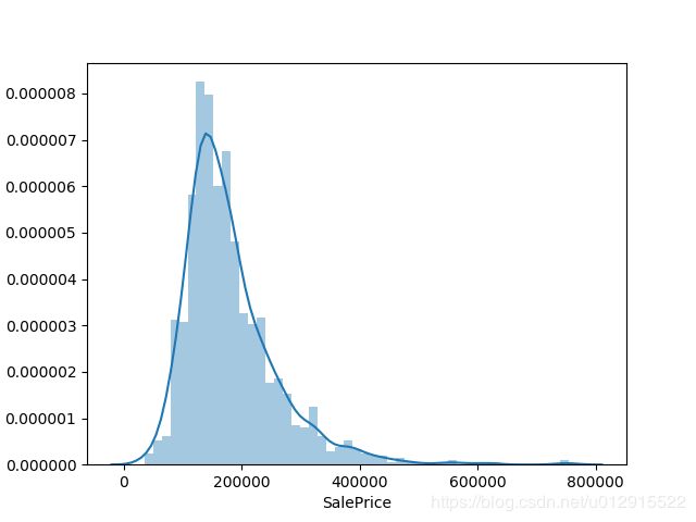
首先观察训练集中售出价格的分布,如下图,典型的右偏分布(即众数<中位数<平均数)。符合一般的认识。
在对特征进行分析之前先将特征归个类别,如下表。
| 类别 | 特征 |
|---|---|
| 住宅概况 | BldgType HouseStyle YearBuilt YearRemodAdd LandContour LandSlope MSSubClass Functional MiscFeature MiscVal |
| 建筑详情 | OverallQual OverallCond RoofStyle RoofMatl Exterior1st Exterior2nd MasVnrType MasVnrArea ExterQual ExterCond 3SsnPorch ScreenPorch EnclosedPorch OpenPorchSF Foundation WoodDeckSF |
| 房间及硬件 | Kitchen KitchenQual Bedroom FullBath HalfBath PoolArea PoolQC Fireplaces FireplaceQu TotRmsAbvGrd Fence |
| 楼层面积 | 1stFlrSF2ndFlrSFLowQualFinSFGrLivArea |
| 地下室相关 | BsmtQual (地下室高度) BsmtCond BsmtExposure BsmtFinType1 BsmtFinSF1 BsmtFinType2 BsmtFinSF2 BsmtUnfSF TotalBsmtSF BsmtFullBath BsmtHalfBath |
| 地块 | LotFrontage LotArea LotShape |
| 交通及环境 | Street Alley MSZoning Neighborhood Utilities PavedDrive Condition1 Condition2 |
| 设备 | Heating HeatingQC Electrical CentralAir |
| 车库 | GarageType GarageYrBlt GarageFinish GarageCars GarageArea GarageCond GarageQual |
| 房屋售出详情 | MoSold YrSold SaleType SaleCondition |
1.2 缺失值分析和处理
将训练集和测试集导入,并检查缺失值的数量:
train_df.T[train_df.isnull().any().values].T.isnull().sum()
test_df.T[test_df.isnull().any().values].T.isnull().sum()
可以得到
LotFrontage      259
Alley           1369
MasVnrType         8
MasVnrArea         8
BsmtQual          37
BsmtCond          37
BsmtExposure      38
BsmtFinType1      37
BsmtFinType2      38
Electrical         1
FireplaceQu      690
GarageType        81
GarageYrBlt       81
GarageFinish      81
GarageQual        81
GarageCond        81
PoolQC          1453
Fence           1179
MiscFeature     1406

MSZoning           4
LotFrontage      227
Alley           1352
Utilities          2
Exterior1st        1
Exterior2nd        1
MasVnrType        16
MasVnrArea        15
BsmtQual          44
BsmtCond          45
BsmtExposure      44
BsmtFinType1      42
BsmtFinSF1         1
BsmtFinType2      42
BsmtFinSF2         1
BsmtUnfSF          1
TotalBsmtSF        1
BsmtFullBath       2
BsmtHalfBath       2
KitchenQual        1
Functional         2
FireplaceQu      730
GarageType        76
GarageYrBlt       78
GarageFinish      78
GarageCars         1
GarageArea         1
GarageQual        78
GarageCond        78
PoolQC          1456
Fence           1169
MiscFeature     1408
SaleType           1
dtype: int64
观察总共有34个特征有缺失值,其中在训练集中有19个特征存在缺失值,测试集有33个特征有缺失值。接下来来具体分析一下各个特征缺失值的具体情况,这里需要用到变量说明data_description.txt。
None
变量说明中可以看到有些类型变量值NA本来就是一个分类值,比如Alley, Basement系列的,FireplaceQu,Garage系列的,PoolQC,Fence,MiscFeature。在这些特征中NA代表着None,而不是缺失值。
Alley: Type of alley access to property

       Grvl	Gravel
       Pave	Paved
       NA 	No alley access

BsmtQual: Evaluates the height of the basement

       Ex	Excellent (100+ inches)
       Gd	Good (90-99 inches)
       TA	Typical (80-89 inches)
       Fa	Fair (70-79 inches)
       Po	Poor (<70 inches
       NA	No Basement

FireplaceQu: Fireplace quality

       Ex	Excellent - Exceptional Masonry Fireplace
       Gd	Good - Masonry Fireplace in main level
       TA	Average - Prefabricated Fireplace in main living area or Masonry Fireplace in basement
       Fa	Fair - Prefabricated Fireplace in basement
       Po	Poor - Ben Franklin Stove
       NA	No Fireplace

GarageType: Garage location

       2Types	More than one type of garage
       Attchd	Attached to home
       Basment	Basement Garage
       BuiltIn	Built-In (Garage part of house - typically has room above garage)
       CarPort	Car Port
       Detchd	Detached from home
       NA	No Garage
0 值
有一些有缺失值的特征应该定义为0,就像如果没有车库,那么相应的车库面积及车库可放车数都应该是0,比如 GarageCars,GarageArea ,BsmtFinSF1,BsmtFinSF2,BsmtUnfSF,TotalBsmtSF,BsmtFullBath,BsmtHalfBath。
Miss
有一些缺失值就是在收集数据的时候漏缺的,可以通过中位数或者众数填充,比如LotFrontage,MasVnrType等。
可以得到一下缺失值表格。
+-------------+-------+-------------+---------------+-------+-------+
train dataset  number    type          test dataset   number   type
+-------------+-------+-------------+---------------+-------+-------+
LotFrontage      259    miss           LotFrontage      227    miss
Alley           1369    None           Alley           1352    None
MasVnrType         8    miss or none   MasVnrType        16    miss or none
MasVnrArea         8    miss or none   MasVnrArea        15    miss or none
BsmtQual          37    None           BsmtQual          44    None
BsmtCond          37    None           BsmtCond          45    None
BsmtExposure      38    None           BsmtExposure      44    None
BsmtFinType1      37    None           BsmtFinType1      42    None
BsmtFinType2      38    None           BsmtFinType2      42    None
Electrical         1    miss
FireplaceQu      690    None           FireplaceQu      730    None
GarageType        81    None           GarageType        76    None
GarageYrBlt       81    None           GarageYrBlt       78    None
GarageFinish      81    None           GarageFinish      78    None
GarageQual        81    None           GarageQual        78    None
GarageCond        81    None           GarageCond        78    None
PoolQC          1453    None           PoolQC          1456    None
Fence           1179    None           Fence           1169    None
MiscFeature     1406    None           MiscFeature     1408    None
                                       MSZoning           4    miss
                                       Utilities          2    miss
                                       Exterior1st        1    miss
                                       Exterior2nd        1    miss
                                       GarageCars         1    may be 0
                                       GarageArea         1    may be 0
                                       BsmtFinSF1         1    may be 0
                                       BsmtFinSF2         1    may be 0
                                       BsmtUnfSF          1    may be 0
                                       TotalBsmtSF        1    may be 0
                                       BsmtFullBath       2    may be 0
                                       BsmtHalfBath       2    may be 0
                                       KitchenQual        1    miss
                                       Functional         2    miss
                                       SaleType           1    miss
处理缺失值
# 针对NA代表None的情况,直接将NA用None替换
train_feature1 = ('Alley', 'BsmtQual', 'BsmtCond', 'BsmtExposure', 'BsmtFinType1', 'BsmtFinType2', 'FireplaceQu',
                  'GarageType', 'GarageYrBlt', 'GarageFinish', 'GarageQual', 'GarageCond', 'PoolQC', 'Fence',
                  'MiscFeature', 'MasVnrType')
test_feature1 = ('Alley', 'BsmtQual', 'BsmtCond', 'BsmtExposure', 'BsmtFinType1', 'BsmtFinType2', 'FireplaceQu',
                 'GarageType', 'GarageYrBlt', 'GarageFinish', 'GarageQual', 'GarageCond', 'PoolQC', 'Fence',
                 'MiscFeature', 'MasVnrType')
for loopi in train_feature1:
    train_df[loopi] = train_df[loopi].fillna('None')
for loopj in test_feature1:
    test_df[loopj] = test_df[loopj].fillna('None')

# 针对NA代表0的情况,直接用0替换
train_df['MasVnrArea'] = train_df['MasVnrArea'].fillna(0)
test_feature2 = ('GarageCars', 'GarageArea', 'BsmtFinSF1', 'BsmtUnfSF', 'TotalBsmtSF', 'BsmtFinSF2', 'BsmtFullBath', 'BsmtHalfBath', 'MasVnrArea')
for loopk in test_feature2:
    test_df[loopk] = test_df[loopk].fillna(0)


# 针对NA代表缺失值,暂采用众数(文本型)或者平均数(数值型)替换
train_df['Electrical'] = train_df['Electrical'].fillna(train_df.Electrical.mode()[0])
test_feature3 = ('MSZoning', 'Utilities', 'KitchenQual', 'Functional', 'SaleType', 'Exterior1st', 'Exterior2nd')
for loopn in test_feature3:
    test_df[loopn] = test_df[loopn].fillna(test_df[loopn].mode()[0])
train_df['LotFrontage'] = train_df['LotFrontage'].fillna(train_df['LotFrontage'].mean())
test_df['LotFrontage'] = test_df['LotFrontage'].fillna(test_df['LotFrontage'].mean())
经过检测,现在样本矩阵中没有缺失值了。
1.3 数值型特征相关性分析
在初始数据中可以看到在79个特征中数值型特征有36个(+2列是Id和SalePrice)。计算相关系数矩阵,并制图如下

从中挑选出有相关系数大于0.5的项组成相关系数子矩阵,如下图所示。
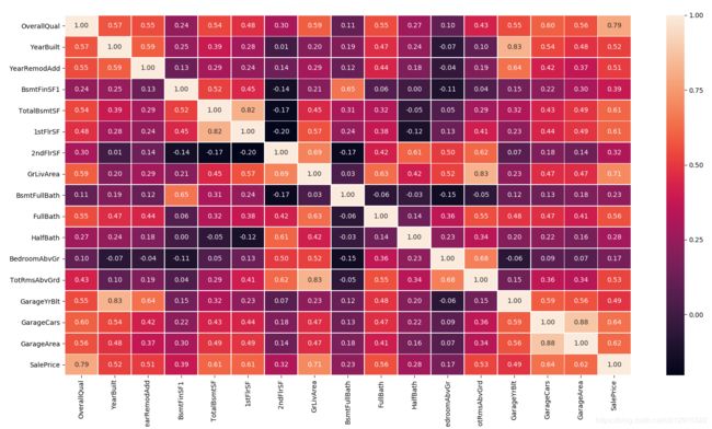
从中可以总结,对于售价影响较大的几点:
- OverallQual(整体材质和竣工质量)与SalePirce的相关系数最高,达到0.79,说明在房屋销售中,大众最关心的还是房屋的质量。
- GrLivArea(地面以上居住面积)与SalePirce的相关系数其次,达到0.71,这个很容易理解,肯定是越大的房子越贵嘛(单价相同的情况下)。
- GarageCars(车库可容纳几辆车)和GarageArea(车库面积)与SalePirce的相关系数也很大,分别是0.64和0.62,说明在美国人心目中车库大小的重要程度。
- TotalBsmtSF(地下室总面积)和1stFlrSF(一楼面积)与SalePirce的相关系数均为0.61,说明美国人把地下室的地位看的很重,与一楼面积同等重要。
当然观察各个因素之间的相关系数,可以发现更多信息,比如:
1.GarageCars与GarageArea相关系数高达0.88,这也可以理解,毕竟车库越大就能放更多车,能放很多车的车库面积自然大;
2.GarageYrBlt与YearBuilt相关系数达到0.83,这也不难理解;
3.TotRmsAbvGrd与GrLivArea相关系数达到0.83,同理面积大了房间就多;
4.其他互相相关系数较高的有(1stFlrSF, TotalBsmtSF)=0.82.
1.4 异常值检测和处理
检测离群值同样重要。由于这个问题中的特征特别的多,所以以与SalePrice相关系数高的几个特征入手,来检测异常值,是一个有用的途径。下图可见在OverallQual中,有许多值在箱型图外面,但是远离的程度并不高,由于还有几个相关系数较高的因素,所以可能在这些样本中由于其他特征使得售价变高了。其中OverallQual=4的样本(40,198)和OverallQual=8的样本(770),但是观察这几个样本的其他特征,比如GrLivArea(40,198,770)=(2287,3112,3279),由于面积大所以贵,还是可以解释的通。

所以先放一放,继续来看GrLivArea与SalePrice的散点图,可以看到整体显示很高的正相关趋势,其中右下角两个样本有点反常,这两个样本是(524,1299),同样查其他特征下的值OverallQual(524,1299)=(10,10),这就有点奇怪了,为啥评价高而且面积达的价格这么低。再看GarageCars(524,1299)=(3,2),同样不错,所以判定这两个样本应该是异常值或者离群值,应该去掉。
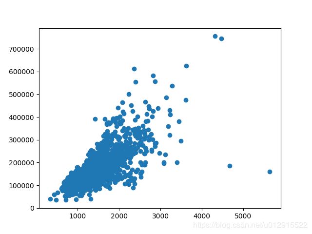
train_df.drop([524,1299], inplace=True)
1.6 去除相关性高的变量
从1.4节中可以看到很多特征相互的相关系数特别高,特征矩阵中去除部分特征以解决这些共线性问题,可以去除一下特征
drop_feature = ('GarageArea', 'GarageYrBlt',  'TotalBsmtSF', 'TotalRmsAbvGrd', 'BsmtFinSF1', '1stFlrSF')
train_df.drop(drop_feature, axis=1, inplace=True)
1.5 数值型转换为分类变量
可以看到其实MSSubClass虽然是数值型变量,但是其实是分类变量,所以将其转换为分类变量
train_df['MSSubClass'] = train_df['MSSubClass'].astype(str)
test_df['MSSubClass'] = test_df['MSSubClass'].astype(str)
1.6 偏态分布转换
我们回忆一下SalePrice的分布,SalePrice是右偏分布。
from scipy.stats import norm
sns.distplot(train_df.SalePrice, fit=norm)
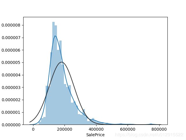

对SalePrice取对数,在来看,基本上符合正态分布。
price = np.log(train_df.SalePrice)

对于数值型其他变量也要做这样的转换
dataset = pd.concat([train_df, test_df])
skew_value = dataset.select_dtypes(include=['int64', 'float']).apply(lambda x: skew(x.dropna()))
skew_df = pd.DataFrame({'Skew':skew_value})
skew_df = skew_df[np.abs(skew_df.Skew)>0.5]
for loopm in skew_df.index.drop('SalePrice').values:
    dataset[loopm] = boxcox1p(dataset[loopm], 0.1)
1.7 分类变量编码
dataset = pd.get_dummis(dataset)
1.8 标准化
sc = RobustScaler()
train_feature = sc.fit_transform(train_feature)
test_feature = sc.transform(test_feature)
2.模型训练及预测
本文采用Lasso模型来预测
# lasso model
model = Lasso(alpha=0.0005, random_state=0)
model.fit(train_feature, price)

predict = model.predict(test_feature)
predicts = np.exp(predict)
output = pd.DataFrame({'Id':test_df.Id, 'SalePrice':predicts})
output.to_csv(r'H:\DataAnalysis\predictprice\regression.csv', index=False)
上传得分为0.11974