Octave 基本操作
Octave 基本操作
- Octave 基本操作
- 简单的运算
- 矩阵相关操作
- 存储和加载数据
- 操作数据
- 绘制图像
- 循环、判断语句
- 函数
- 退出
Octave 基本操作
学习Andrew ng的machine learning课程,初步接触了Octave,总结一下Octave的基本操作。
原课程链接
简单的运算
我们对Markdown编辑器进行了一些功能拓展与语法支持,除了标准的Markdown编辑器功能,我们增加了如下几点新功能,帮助你用它写博客:
- 算术运算
>>  5+6
ans =  11
>> 3-2
ans =  1
>> 1/2
ans =  0.50000
>> 2^6
ans =  64
- 逻辑运算
result 0-false
1-true
>> 1>2
ans = 0
>> 2>1
ans = 1
>> 1==2
ans = 0
>> 1~=2
ans = 1
>> 1&&0
ans = 0
>> 1||0
ans = 1
>> xor(1,0)  %异或
ans = 1
>> a = 3
a =  3
>> a =3;  %加分号后结果不显示

>> b = 'hi';
>> b
b = hi

>> c =( 3>=1)
c = 1  % c为true
- 输出打印命令
>> a=pi
a =  3.1416
>> a = pi;
>> disp(a)
 3.1416

>> disp(sprintf('6 decimals:%0.6f',a))
6 decimals:3.141593

>> disp(sprintf('2 decimals:%0.2f',a))
2 decimals:3.14
- 浮点数格式转换
>> a
a =  3.1416
>> format long
>> a
a =  3.141592653589793
>> format short
>> a
a =  3.1416
>>
矩阵相关操作
- 定义并赋值
>> A = [1 2;3 4;5 6]
A =

   1   2
   3   4
   5   6

>> B = [1 2;
3 4;
5 6;
7 8]
B =

   1   2
   3   4
   5   6
   7   8


>> V = [1 2 3]  % 行向量
V =

   1   2   3

>> Q = [1;2;3] % 列向量
Q =

   1
   2
   3

>>
>> V = 1:0.1:2
V =

 Columns 1 through 9:

    1.0000    1.1000    1.2000    1.3000    1.4000    1.5000    1.6000    1.7000    1.8000

 Columns 10 and 11:

    1.9000    2.0000
>> V = 1:6
V =

   1   2   3   4   5   6

>>
- . 生成特殊矩阵的快捷命令
ones(x,y) 生成x行y列元素全1的矩阵
zeros(x,y) 生成x行y列元素全0的矩阵
rand(x,y) 生成x行y列元素介于0到1之间的随机数矩阵
randn(x,y) 生成x行y列,元素平均值为0的高斯分布矩阵
eye(n) 生成n阶单位矩阵
>> ones(2,3)
ans =

   1   1   1
   1   1   1

>> C = 2*ones(2,3)
C =

   2   2   2
   2   2   2

>> W = ones(1,3)
W =

   1   1   1
>> W = zeros(1,3)
W =

   0   0   0

>> W= rand(2,3)
W =

   0.427168   0.130783   0.079716
   0.775599   0.096085   0.104985

>>
>> W = randn(1,3)
W =

  -1.835300  -0.041527   0.829504
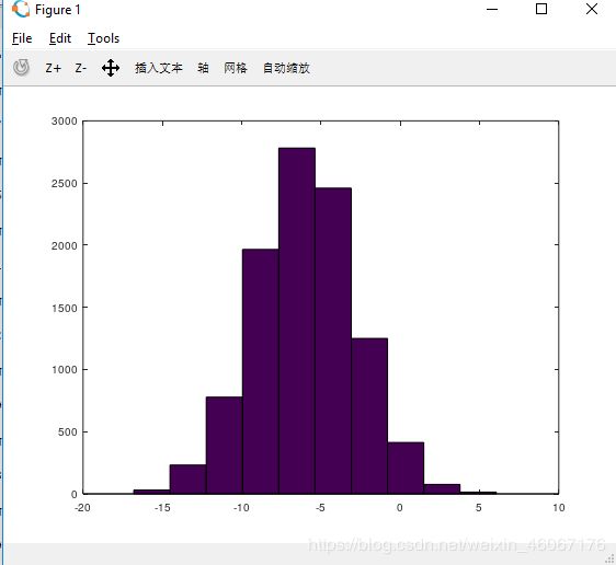
W = -6 +sqrt(10)*(randn(1,10000))
>> eye(4)
ans =

Diagonal Matrix

   1   0   0   0
   0   1   0   0
   0   0   1   0
   0   0   0   1

>>
3. 矩阵的基本操作
>> A
A =

   1   2
   3   4
   5   6

>> size(A)
ans =

   3   2
>> size(A,1)
ans =  3
>> size(A,2)
ans =  2
>> V = [1 2 3 4]
V =

   1   2   3   4


>> length(V)
ans =  4
>> length(A)  %返回最大的维度
ans =  3
4 画图
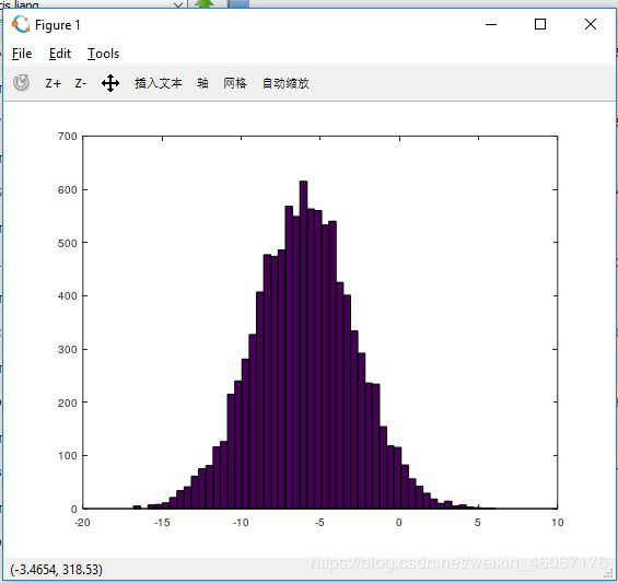
>> hist(W)
>> hist(W,50)
5. 帮助命令
>> help eye
'eye' is a built-in function from the file libinterp/corefcn/data.cc

 -- eye (N)
 -- eye (M, N)
 -- eye ([M N])
 -- eye (..., CLASS)
     Return an identity matrix.

     If invoked with a single scalar argument N, return a square NxN
     identity matrix.

     If supplied two scalar arguments (M, N), 'eye' takes them to be the
     number of rows and columns.  If given a vector with two elements,
     'eye' uses the values of the elements as the number of rows and
     columns, respectively.  For example:

          eye (3)
           =>  1  0  0
               0  1  0
               0  0  1

     The following expressions all produce the same result:

          eye (2)
          ==
          eye (2, 2)
          ==
          eye (size ([1, 2; 3, 4]))

     The optional argument CLASS, allows 'eye' to return an array of the
     specified type, like

          val = zeros (n,m, "uint8")

     Calling 'eye' with no arguments is equivalent to calling it with an
     argument of 1.  Any negative dimensions are treated as zero.  These
     odd definitions are for compatibility with MATLAB.

     See also: speye, ones, zeros.

Additional help for built-in functions and operators is
available in the online version of the manual.  Use the command
'doc <topic>' to search the manual index.

Help and information about Octave is also available on the WWW
at https://www.octave.org and via the [email protected]
mailing list.
存储和加载数据
>> cd 'd:\'
>> pwd
ans = d:\
>> ls  %查找文件
>> load xxxx.dat %加载数据文件
>> load ('xxxx.dat') %用法同上
>> who  %查看当前定义的变量
Variables in the current scope:

A    B    C    Q    V    W    a    ans  b    c
>> whos
Variables in the current scope:

   Attr Name        Size                     Bytes  Class
   ==== ====        ====                     =====  =====
        A           3x2                         48  double
        B           3x2                         48  double
        C           2x3                         48  double
        Q           3x1                         24  double
        V           1x4                         32  double
        W           1x10000                  80000  double
        a           1x1                          8  double
        ans         1x3                          3  char
        b           1x2                          2  char
        c           1x1                          1  logical

Total is 10032 elements using 80214 bytes
>> clear A
>> whos
Variables in the current scope:

   Attr Name        Size                     Bytes  Class
   ==== ====        ====                     =====  =====
        B           3x2                         48  double
        C           2x3                         48  double
        Q           3x1                         24  double
        V           1x4                         32  double
        W           1x10000                  80000  double
        a           1x1                          8  double
        ans         1x3                          3  char
        b           1x2                          2  char
        c           1x1                          1  logical

Total is 10026 elements using 80166 bytes
>> VV = V(1:2)
VV =

   1   2

>> V
V =

   1   2   3   4

>> save hello.mat VV  %保存文件

>> clear
>> whos
>> load hello.mat
>> whos
Variables in the current scope:

   Attr Name        Size                     Bytes  Class
   ==== ====        ====                     =====  =====
        VV          1x2                         16  double

Total is 2 elements using 16 bytes
>> save hello.txt -ascii
操作数据
>> A =[1 2;3 4; 5 6]
A =

   1   2
   3   4
   5   6

>> A(3,2)
ans =  6
>> A(2,:)   % "%" means every element alont that row/column
ans =

   3   4
>> A(:,2)
ans =

   2
   4
   6
>> A([1 3],:) %第一列和第三列所有
ans =

   1   2
   5   6
>> A(:,2)=[10; 11; 12]
A =

    1   10
    3   11
    5   12
>> A =[A,[100;101;102]]
A =

     1    10   100
     3    11   101
     5    12   102
>> A(:)  %put all elements of A into a single vector
ans =

     1
     3
     5
    10
    11
    12
   100
   101
   102
>> A = [1 2;3 4;5 6]
A =

   1   2
   3   4
   5   6

>> B
B =

   10   11
   12   13
   14   15

>> C = [A,B]
C =

    1    2   10   11
    3    4   12   13
    5    6   14   15

>> D = [A;B]
D =

    1    2
    3    4
    5    6
   10   11
   12   13
   14   15

>> A = [1 2;3 4;5 6]
A =

   1   2
   3   4
   5   6

>> B = [11 12;13 14;15 16]
B =

   11   12
   13   14
   15   16

>> A .* B  %每个对应元素相乘
ans =

   11   24
   39   56
   75   96
>> A .^2
ans =

    1    4
    9   16
   25   36

>> V = [1;2;3]
V =

   1
   2
   3

>> 1 ./V
ans =

   1.00000
   0.50000
   0.33333

>> 1 ./A
ans =

   1.00000   0.50000
   0.33333   0.25000
   0.20000   0.16667

>> log(V)      %以e为底的对数运算
ans =

   0.00000
   0.69315
   1.09861

>> exp(V)    %e的幂次运算
ans =

    2.7183
    7.3891
   20.0855
>> abs([-1;2;-3])  %绝对值
ans =

   1
   2
   3
>> -V
ans =

  -1
  -2
  -3
>> V + ones(length(V),1)
ans =

   2
   3
   4
ᴬ>> A
A =
1 2
3 4
5 6
>> A' %转置
ans =
1 3 5
2 4 6
>> a = [1 15 2 0.5]
a =
1.00000 15.00000 2.00000 0.50000
>> val = max(a)
val = 15
>> [val, ind] = max(a) %找出最大值和最大值的索引
val = 15
ind = 2
>> a
a =
1.00000 15.00000 2.00000 0.50000
>> a < 3 %每个元素小于3,true or false
ans =
1 0 1 1
A =
1 100
2 3
4 5
>> find (a <3) %小于3的元素的index
ans =
1 3 4
>> max(A)
ans =
4 100
>> magic(3) %每行每列加一起和相等
ans =
8 1 6
3 5 7
4 9 2
>> A = magic(3)
A =
8 1 6
3 5 7
4 9 2
>> [r,c]=find(A >=7)
r =
1
3
2
c =
1
2
3
>> A
A =

   8   1   6
   3   5   7
   4   9   2

>> max(A)
ans =

   8   9   7

>> max(max(A))
ans =  9
>> max(A,[],1)
ans =

   8   9   7

>> max(A,[],2)
ans =

   8
   7
   9
>> max(A(:))
ans =  9
>> a
a =

    1.00000   15.00000    2.00000    0.50000

>> sum(a)
ans =  18.500
>> prod(a)
ans =  15
>> floor(a)
ans =

    1   15    2    0

>> ceil(a)
ans =

    1   15    2    1
>> A
A =

   8   1   6
   3   5   7
   4   9   2

>> pinv(A)   %逆矩阵
ans =

   0.147222  -0.144444   0.063889
  -0.061111   0.022222   0.105556
  -0.019444   0.188889  -0.102778

 - [ ] List item
绘制图像
>> t=[0:0.01:0.98]
t =
Columns 1 through 15:
0.00000 0.01000 0.02000 0.03000 0.04000 0.05000 0.06000 0.07000 0.08000 0.09000 0.10000 0.11000 0.12000 0.13000 0.14000
Columns 16 through 30:
0.15000 0.16000 0.17000 0.18000 0.19000 0.20000 0.21000 0.22000 0.23000 0.24000 0.25000 0.26000 0.27000 0.28000 0.29000
Columns 31 through 45:
0.30000 0.31000 0.32000 0.33000 0.34000 0.35000 0.36000 0.37000 0.38000 0.39000 0.40000 0.41000 0.42000 0.43000 0.44000
Columns 46 through 60:
0.45000 0.46000 0.47000 0.48000 0.49000 0.50000 0.51000 0.52000 0.53000 0.54000 0.55000 0.56000 0.57000 0.58000 0.59000
Columns 61 through 75:
0.60000 0.61000 0.62000 0.63000 0.64000 0.65000 0.66000 0.67000 0.68000 0.69000 0.70000 0.71000 0.72000 0.73000 0.74000
Columns 76 through 90:
0.75000 0.76000 0.77000 0.78000 0.79000 0.80000 0.81000 0.82000 0.83000 0.84000 0.85000 0.86000 0.87000 0.88000 0.89000
Columns 91 through 99:
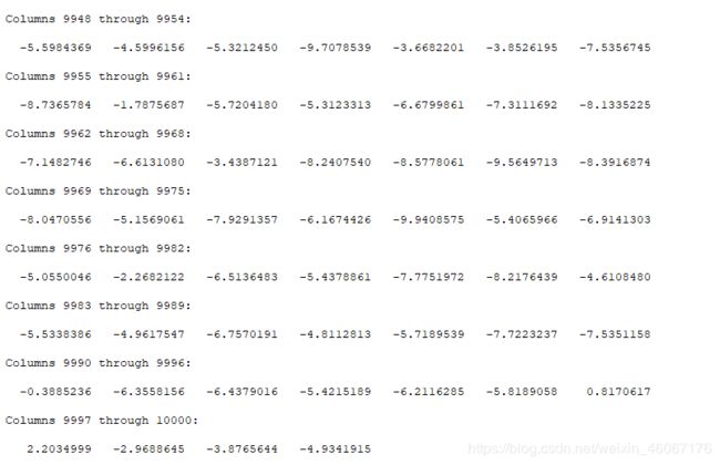
0.90000 0.91000 0.92000 0.93000 0.94000 0.95000 0.96000 0.97000 0.98000
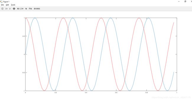
>> y1 = sin(2*pi*4*t);
>> plot(t,y1)
>> y2 = cos(2*pi*4*t);
>> plot(t,y2)
>> plot(t,y1)
>> hold on
>> plot(t,y2,'r')
>> xlabel('time')
>> ylabel('value')
>> legend('sin','cos')   %设置图例
>> title('my plot')
>> cd 'D:\' ; print -dpng 'myPlot.png'  %保存图像
>> close  %关闭图像

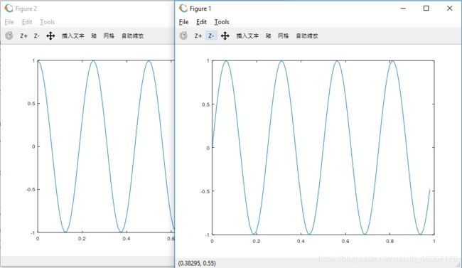
>> figure(1); plot(t,y1)
>> figure(2); plot(t,y2)  %新开一个名为figure2的窗口,绘制第二个图
>> subplot(1,2,1) %将画布分为1X2的格子,访问第一个格子
>> plot(t,y1)   %图像会出现在第一个格子里
>> subplot(1,2,2)  %访问第二个格子
>> plot(t,y2)        %图像会出现在第二个格子里
>> axis([0.5 1 -1 1])  %改变x y轴的范围


>> A = magic(5)
A =

   17   24    1    8   15
   23    5    7   14   16
    4    6   13   20   22
   10   12   19   21    3
   11   18   25    2    9

>> imagesc(A)
>> imagesc(A), colorbar, colormap grey;


循环、判断语句
>> V = zeros(10,1)
V =

   0
   0
   0
   0
   0
   0
   0
   0
   0
   0

>> for i=1:10,
    V(i)=2^i
end;

V =

      2
      4
      8
     16
     32
     64
    128
    256
    512
   1024
>> i = 1;
>> while i<=5,
    V(i) = 100,
    i = i+1,
end;

V =

    100
    100
    100
    100
    100
     64
    128>> i = 1,
i =  1
>> while true,
     V(i) = 99,
     i = i+1;
     if i == 6,
       break;
  end;
end
    256
    512
   1024


V =

     99
     99
     99
     99
     99
     64
    128
    256
    512
   1024
>> V(1)
ans =  99
>> V(1)=2
V =

      2
     99
     99
     99
     99
     64
    128
    256
    512
   1024

>> if V(1) == 1,
     disp('The value is one')
   elseif V(1) ==2,
     disp('The value is two')
   else
     disp('The value is not one or two')
end;
The value is two
函数
保存在xx.m的函数文件里
function y =  squareThisNumber(x)

y = x^2;
调用
>> cd 'D:\Octave-5.2.0\functions'
>> pwd
ans = D:\Octave-5.2.0\functions
>> squareThisNumber(3)
ans =  9

>> addpath('')  %将路径加入octave search  path
Octave中函数可以返回多个值
退出
>> exit
>> quit