IsolationForest-02Python案例

Intro

  sklearn中IsolationForest使用，包括参数说明和实际案例。
  简述下算法思想： 随机选择特征，在该特征的maximum和minimum中随机选择切分值(split value)。如此递归划分，形成树。根节点到终止节点(叶子结点)的长度，等价于split的次数。对于多棵树，计算平均长度，可以反映样本异常的程度。即异常样本通常较快被划分到叶子结点，因而路径长度较小。

slearn版本:0.22

import sklearn
sklearn.__version__

'0.22'

参数介绍

Parameters

n_estimators:int, optional (default=100)
//树的棵数，paper中建议100棵，再增加模型效果提升有限//
 The number of base estimators in the ensemble.

max_samples:int or float, optional (default=”auto”)
//sunsample样本大小，默认256，如果是int，则抽取样本数为该值；如果是float，按照比例计算即可//
 The number of samples to draw from X to train each base estimator.

• If int, then draw max_samples samples.
• If float, then draw max_samples * X.shape[0] samples.
• If “auto”, then max_samples=min(256, n_samples).

 If max_samples is larger than the number of samples provided, all samples will be used for all trees (no sampling).

contamination:‘auto’ or float, optional (default=‘auto’)
//样本中离群值的占比，默认"auto"是采用paper中的阈值，paper似乎没有提阈值，sklearn是0.5；float则自己指定，范围[0,0.5]，这里float是分位数的意思，0.25就是得到所有得分，计算25%分位数 //
 The amount of contamination of the data set, i.e. the proportion of outliers in the data set. Used when fitting to define the threshold on the scores of the samples.

• If ‘auto’, the threshold is determined as in the original paper.
• If float, the contamination should be in the range [0, 0.5].

max_features:int or float, optional (default=1.0)
//每棵树训练时，参与分裂的树的特征数，默认是1，代码里看好像是不用进行列抽样，但是bagging那里的代码没怎么看懂~ //
 The number of features to draw from X to train each base estimator.

• If int, then draw max_features features.
• If float, then draw max_features * X.shape[1] features.

bootstrap:bool, optional (default=False)
//subsample时，采取有放回抽样还是无放回,默认不放回 //
If True, individual trees are fit on random subsets of the training data sampled with replacement. If False, sampling without replacement is performed.

n_jobs:int or None, optional (default=None)
//模型训练和预测时，工作的core数量，-1则全部用来工作//
The number of jobs to run in parallel for both fit and predict. None means 1 unless in a joblib.parallel_backend context. -1 means using all processors. See Glossary for more details.

random_state:int, RandomState instance or None, optional (default=None)
//设置随机数，方便结果可复现//

• If int, random_state is the seed used by the random number generator
• If RandomState instance, random_state is the random number generator
• If None, the random number generator is the RandomState instance used by np.random

verbose:int, optional (default=0)
//树的构建过程是否输出？？//
Controls the verbosity of the tree building process.

warm_start:bool, optional (default=False)
//参考这里吧，我是没看懂 https://scikit-learn.org/stable/glossary.html#term-warm-start//
When set to True, reuse the solution of the previous call to fit and add more estimators to the ensemble, otherwise, just fit a whole new forest. See the Glossary.

Attributes

estimators_:list of DecisionTreeClassifier
The collection of fitted sub-estimators.

estimators_samples_:list of arrays
The subset of drawn samples for each base estimator.

max_samples_:integer
The actual number of samples

offset_:float
Offset used to define the decision function from the raw scores. We have the relation: decision_function = score_samples - offset_. offset_ is defined as follows. When the contamination parameter is set to “auto”, the offset is equal to -0.5 as the scores of inliers are close to 0 and the scores of outliers are close to -1. When a contamination parameter different than “auto” is provided, the offset is defined in such a way we obtain the expected number of outliers (samples with decision function < 0) in training.

Methods

////
decision_function(self, X)
//返回基学习器的平均得分=score_samples-offset；得分越低越不正常//
Average anomaly score of X of the base classifiers.

fit(self, X[, y, sample_weight])
//拟合模型//
Fit estimator.

fit_predict(self, X[, y])
//预测//
Perform fit on X and returns labels for X.

get_params(self[, deep])
//得到模型参数//
Get parameters for this estimator.

predict(self, X)
//预测//
Predict if a particular sample is an outlier or not.

score_samples(self, X)
//得分，计算逻辑得看下代码和paper//
Opposite of the anomaly score defined in the original paper.

set_params(self, **params)
//设置参数//
Set the parameters of this estimator.

Demo

Copy文档里简单的一维数据进行测试，查看各个方法输出的结果

import numpy as np
from sklearn.ensemble import IsolationForest
from sklearn.ensemble import _average_path_length
X = [[-1.1], [0.3], [0.5], [100]]
clf1 = IsolationForest(random_state=0)
clf1.fit(X)
clf2 = IsolationForest(random_state=0,contamination=0.1)
clf2.fit(X)

IsolationForest(behaviour='deprecated', bootstrap=False, contamination=0.1,
                max_features=1.0, max_samples='auto', n_estimators=100,
                n_jobs=None, random_state=0, verbose=0, warm_start=False)

模型的参数

clf1.get_params()

{'behaviour': 'deprecated',
 'bootstrap': False,
 'contamination': 'auto',
 'max_features': 1.0,
 'max_samples': 'auto',
 'n_estimators': 100,
 'n_jobs': None,
 'random_state': 0,
 'verbose': 0,
 'warm_start': False}

预测得分

得分相关的方法有四个：

• _compute_score_samples: 返回结果记score1，和paper里score的计算逻辑一致
• _compute_chunked_score_samples:返回结果记score2，和paper里score的计算逻辑一致，且score1=score2
• score_samples:返回结果记score3，对_compute_score_samples结果取相反数,即-score3=score2=score1
• decision_function:score_samples返回结果-offset,其中offset默认为-0.5，如果contamination为float，比如0.1，那么offset为score3的10%分位数

clf1._compute_score_samples(np.asarray(X),False)

array([0.46946339, 0.32529681, 0.33144271, 0.68006339])

clf1._compute_chunked_score_samples(np.asarray(X))

array([0.46946339, 0.32529681, 0.33144271, 0.68006339])

clf1.score_samples(X)

array([-0.46946339, -0.32529681, -0.33144271, -0.68006339])

clf1.decision_function(X)

array([ 0.03053661,  0.17470319,  0.16855729, -0.18006339])

clf1.score_samples(X)-(-0.5)

array([ 0.03053661,  0.17470319,  0.16855729, -0.18006339])

预测标签

打标逻辑：decision_function小于0的就是异常样本

 clf1.predict(X)

array([ 1,  1,  1, -1])

offset计算逻辑

  offset和contamination参数有关，"auto"是为-0.5，否则通过float类型计算分位数

clf2.offset_

-0.6168833934367299

np.percentile(clf2.score_samples(X),100. *0.1)

-0.6168833934367299

Case 1

构造数据

import numpy as np
import matplotlib.pyplot as plt
from sklearn.ensemble import IsolationForest
# 随机数相关，后期用来构造测试数据
rng = np.random.RandomState(42)
# Generate train data
# 生成100行2列array的0-1随机数，并且乘0.3，映射值域到[0,0.3] 
X = 0.3 * rng.randn(100, 2)
# 对X分别加减2，得到两个(100,2)的矩阵
# 通过np.r_，对两个矩阵行合并，类似R里的rbind  
X_train = np.r_[X + 2, X - 2]
# Generate some regular novel observations
# 下面生成测试数据，分布和生成逻辑保持一致  
X1 = 0.3 * rng.randn(20, 2)
X_test = np.r_[X1 + 2, X1 - 2]
# Generate some abnormal novel observations
# 异常值由均匀分布U(-4,4)构造，20行2列的array  
X_outliers = rng.uniform(low=-4, high=4, size=(20, 2))

模型拟合

# fit the model
clf = IsolationForest(max_samples=100, random_state=rng)
clf.fit(X_train)
y_pred_train = clf.predict(X_train)
y_pred_test = clf.predict(X_test)
y_pred_outliers = clf.predict(X_outliers)

查看结果

print("------ _compute_score_samples ------"+"\n");print(clf._compute_score_samples(np.asarray(X),False)[1:10])
print("------ _compute_chunked_score_samples ------"+"\n");print(clf._compute_chunked_score_samples(np.asarray(X))[1:10])
print("------ score_samples ------"+"\n");print(clf.score_samples(X)[1:10])
print("------ decision_function ------"+"\n");print(clf.decision_function(X)[1:10])

------ _compute_score_samples ------

[0.66061839 0.65897815 0.65788691 0.66281174 0.65897815 0.66289298
 0.66678221 0.66171416 0.66163282]
------ _compute_chunked_score_samples ------

[0.66061839 0.65897815 0.65788691 0.66281174 0.65897815 0.66289298
 0.66678221 0.66171416 0.66163282]
------ score_samples ------

[-0.66061839 -0.65897815 -0.65788691 -0.66281174 -0.65897815 -0.66289298
 -0.66678221 -0.66171416 -0.66163282]
------ decision_function ------

[-0.16061839 -0.15897815 -0.15788691 -0.16281174 -0.15897815 -0.16289298
 -0.16678221 -0.16171416 -0.16163282]

y_pred_train

array([ 1, -1,  1, -1,  1,  1, -1, -1,  1, -1, -1,  1,  1,  1,  1, -1,  1,
       -1, -1,  1,  1,  1, -1,  1, -1,  1,  1, -1,  1,  1,  1, -1, -1,  1,
        1, -1,  1, -1,  1, -1,  1, -1,  1,  1,  1,  1,  1, -1,  1,  1,  1,
        1,  1, -1,  1, -1, -1,  1,  1, -1,  1, -1, -1,  1,  1, -1,  1, -1,
        1, -1,  1, -1,  1, -1,  1,  1,  1,  1, -1,  1,  1, -1, -1, -1,  1,
        1,  1,  1,  1, -1,  1,  1,  1,  1, -1,  1,  1,  1,  1,  1,  1, -1,
        1, -1,  1,  1, -1, -1,  1, -1, -1, -1,  1,  1,  1, -1,  1, -1, -1,
       -1,  1,  1, -1,  1, -1,  1,  1, -1,  1,  1,  1, -1, -1,  1,  1, -1,
       -1, -1,  1, -1,  1, -1,  1,  1,  1,  1,  1, -1,  1,  1, -1,  1,  1,
       -1,  1, -1, -1,  1,  1, -1,  1, -1, -1, -1,  1, -1,  1, -1,  1, -1,
        1, -1,  1, -1,  1,  1,  1,  1, -1, -1,  1, -1, -1, -1,  1, -1,  1,
        1, -1, -1,  1,  1,  1,  1, -1,  1,  1,  1,  1,  1])

可视化

# plot the line, the samples, and the nearest vectors to the plane
# 
xx, yy = np.meshgrid(np.linspace(-5, 5, 50), np.linspace(-5, 5, 50))
# xx.ravel()转成1维
# np.c_列拼接cbind
Z = clf.decision_function(np.c_[xx.ravel(), yy.ravel()])
# 重塑
Z = Z.reshape(xx.shape)

plt.title("IsolationForest")
plt.contourf(xx, yy, Z, cmap=plt.cm.Blues_r)

# 白色的点为train
b1 = plt.scatter(X_train[:, 0], X_train[:, 1], c='white',
                 s=20, edgecolor='k')
# 绿色的点为test
b2 = plt.scatter(X_test[:, 0], X_test[:, 1], c='yellow',
                 s=20, edgecolor='k')
# 红色点为outliers
c = plt.scatter(X_outliers[:, 0], X_outliers[:, 1], c='red',
                s=20, edgecolor='k')
plt.axis('tight')
plt.xlim((-5, 5))
plt.ylim((-5, 5))
plt.legend([b1, b2, c],
           ["training observations",
            "new regular observations", "new abnormal observations"],
           loc="upper left")
plt.show()

  从上面的图来看，红色的异常点，确实大部分分布在簇之外，但是如果从预测的结果看，簇中很多点，也被标记为异常值.总之，感觉iforest的说服力不是很够，最终还是需要人工check，不知道在业界是怎么玩滴。
  https://scikit-learn.org/stable/auto_examples/plot_anomaly_comparison.html#sphx-glr-auto-examples-plot-anomaly-comparison-py介绍了多种算法的比较可以再关注下，或者Paper里用多个数据，通过AUC这个指标进行测试，也可以复现下试试看

Case2-Credit Card Fraud Detection

Intro

  使用kaggle的信用卡盗刷数据，检验iForest效果。数据为信用卡的交易记录，共计284,807条，其中492条盗刷行为，占比0.172%。提供的数据是脱敏之后的，由pca提供的数据，全部都是数值型，也没有缺失值，很适合做无监督的测试。

  不同算法效果比较，通过5折交叉验证，采用AUC，其余指标和阈值有关系，不适合直接比较。为了保证结果可复现，需要控制两个随机性：

• 5折交叉验证时，数据集划分的随机性
• 模型训练时的随机性

EDA

  简单的EDA，对数据做简单探索。

import pandas as pd
import numpy as np
import warnings
warnings.filterwarnings('ignore')

rawdata = pd.read_csv("../Data/creditcard.csv")

rawdata.head()

	Time	V1	V2	V3	V4	V5	V6	V7	V8	V9	...	V21	V22	V23	V24	V25	V26	V27	V28	Amount	Class
0	0.0	-1.359807	-0.072781	2.536347	1.378155	-0.338321	0.462388	0.239599	0.098698	0.363787	...	-0.018307	0.277838	-0.110474	0.066928	0.128539	-0.189115	0.133558	-0.021053	149.62	0
1	0.0	1.191857	0.266151	0.166480	0.448154	0.060018	-0.082361	-0.078803	0.085102	-0.255425	...	-0.225775	-0.638672	0.101288	-0.339846	0.167170	0.125895	-0.008983	0.014724	2.69	0
2	1.0	-1.358354	-1.340163	1.773209	0.379780	-0.503198	1.800499	0.791461	0.247676	-1.514654	...	0.247998	0.771679	0.909412	-0.689281	-0.327642	-0.139097	-0.055353	-0.059752	378.66	0
3	1.0	-0.966272	-0.185226	1.792993	-0.863291	-0.010309	1.247203	0.237609	0.377436	-1.387024	...	-0.108300	0.005274	-0.190321	-1.175575	0.647376	-0.221929	0.062723	0.061458	123.50	0
4	2.0	-1.158233	0.877737	1.548718	0.403034	-0.407193	0.095921	0.592941	-0.270533	0.817739	...	-0.009431	0.798278	-0.137458	0.141267	-0.206010	0.502292	0.219422	0.215153	69.99	0

5 rows × 31 columns

rawdata.shape

(284807, 31)

rawdata.Class.value_counts()

0    284315
1       492
Name: Class, dtype: int64

rawdata.isna().sum()

Time      0
V1        0
V2        0
V3        0
V4        0
V5        0
V6        0
V7        0
V8        0
V9        0
V10       0
V11       0
V12       0
V13       0
V14       0
V15       0
V16       0
V17       0
V18       0
V19       0
V20       0
V21       0
V22       0
V23       0
V24       0
V25       0
V26       0
V27       0
V28       0
Amount    0
Class     0
dtype: int64

• 数据维度:284807行,31列
• 正负样本分布:0-284315;1-492
• 所有列均无缺失值

不做其他数据探索，直接上算法

数据准备

  为了保证数据可比和可重复，交叉验证的数据划分和模型训练需要指定随机数种子。

from sklearn.model_selection import train_test_split, cross_val_score, GridSearchCV,StratifiedKFold

rawdata['Hour'] =rawdata["Time"].apply(lambda x : divmod(x, 3600)[0])
# 特征数据单独存放  
X=rawdata.drop(['Time','Class'],axis=1)
# label数据单独存放  
y=rawdata.Class

X.shape

(284807, 30)

训练、测试数据划分

调用train_test_split函数划分训练集和测试集，设置参数stratify=y，保证划分之后正负样本比和总体样本保持一致。

train_test_split用法 https://scikit-learn.org/stable/modules/generated/sklearn.model_selection.train_test_split.html#sklearn.model_selection.train_test_split

X_traintotal,X_test,y_traintotal,y_test=train_test_split(X,y,stratify=y,test_size=0.2,random_state =12345) 

y_traintotal.value_counts()

0    227451
1       394
Name: Class, dtype: int64

y_test.value_counts()

0    56864
1       98
Name: Class, dtype: int64

5折划分

StratifiedKFold同样可以保证各个折的数据中，正负样本分布和总体一致
StratifiedKFold https://scikit-learn.org/stable/modules/generated/sklearn.model_selection.StratifiedKFold.html#sklearn.model_selection.StratifiedKFold

splits为生成器，只能访问一次。
//假如我们要生成从 1 到 10 这 10 个数字，采用列表的方式定义，会占用 10 个地址空间。采用生成器，只会占用一个地址空间。因为生成器并没有把所有的值存在内存中，而是在运行时生成值。所以生成器只能访问一次。//

NFOLDS = 5
folds = StratifiedKFold(n_splits=NFOLDS,random_state=12345)
splits = folds.split(X_traintotal, y_traintotal)

enumerate函数用法:https://www.runoob.com/python/python-func-enumerate.html
就是给可遍历的数据对象组合成一个索引序列

新建一个list，把K折数据拼接成字典放进去

kFoldsList = []
for fold_n, (train_index, valid_index) in enumerate(splits):
    kFoldsList.append({
        "fold": fold_n,
        "train_index": train_index,
        "valid_index": valid_index
    })

kFoldsList

[{'fold': 0,
  'train_index': array([ 40589,  41263,  41754, ..., 227842, 227843, 227844]),
  'valid_index': array([    0,     1,     2, ..., 45571, 45572, 45573])},
 {'fold': 1,
  'train_index': array([     0,      1,      2, ..., 227842, 227843, 227844]),
  'valid_index': array([40589, 41263, 41754, ..., 91141, 91142, 91143])},
 {'fold': 2,
  'train_index': array([     0,      1,      2, ..., 227842, 227843, 227844]),
  'valid_index': array([ 87243,  87254,  87884, ..., 136716, 136717, 136718])},
 {'fold': 3,
  'train_index': array([     0,      1,      2, ..., 227842, 227843, 227844]),
  'valid_index': array([133467, 133512, 134189, ..., 182282, 182283, 182284])},
 {'fold': 4,
  'train_index': array([     0,      1,      2, ..., 182282, 182283, 182284]),
  'valid_index': array([177302, 177309, 178759, ..., 227842, 227843, 227844])}]

查看下正负样本比

for i in range(len(kFoldsList)):
    print("--- 第"+str(i)+"折数据 ---")
    validY = y_traintotal[kFoldsList[i]["valid_index"]]
    print("      --- 正负样本比: ",str(validY.sum()/validY.count()))

--- 第0折数据 ---
      --- 正负样本比:  0.003181219833260202
--- 第1折数据 ---
      --- 正负样本比:  0.0014567242943132781
--- 第2折数据 ---
      --- 正负样本比:  0.0009863824423925254
--- 第3折数据 ---
      --- 正负样本比:  0.0023323455164087365
--- 第4折数据 ---
      --- 正负样本比:  0.0011241808560225933

下面查看k折的效果，主要关注以下几个方便:

• valid折数据拼起来是否是原始数据的全集
• 每一折数据的train和valid是否都没有交集且并集是原始数据的全集

for i in range(len(kFoldsList)):
    print("------ 第%d折验证集索引 ------"%i)
    print("      --- top3: %s"% str(kFoldsList[i]["valid_index"][0:3]))
    print("      --- tail3: %s"% str(kFoldsList[i]["valid_index"][-3:]))

------ 第0折验证集索引 ------
      --- top3: [0 1 2]
      --- tail3: [45571 45572 45573]
------ 第1折验证集索引 ------
      --- top3: [40589 41263 41754]
      --- tail3: [91141 91142 91143]
------ 第2折验证集索引 ------
      --- top3: [87243 87254 87884]
      --- tail3: [136716 136717 136718]
------ 第3折验证集索引 ------
      --- top3: [133467 133512 134189]
      --- tail3: [182282 182283 182284]
------ 第4折验证集索引 ------
      --- top3: [177302 177309 178759]
      --- tail3: [227842 227843 227844]

validTestList = []
for i in kFoldsList:
    validTestList.extend(i["valid_index"])

set(range(len(X_traintotal)))-set(validTestList)

set()

数据没有问题

LR Baseline

  训练LR模型，和iForest比较。采用5折交叉验证，比较指标选取AUC。

from sklearn.linear_model import LogisticRegression
from sklearn.metrics import roc_auc_score, roc_curve, precision_score, auc, precision_recall_curve, accuracy_score, recall_score, f1_score, confusion_matrix, classification_report

columns = X_traintotal.columns
y_preds = np.zeros(X_test.shape[0])
# 类似rf的带外误差估计，把valid的那一折数据放在这个变量中
y_oof = np.zeros(X_traintotal.shape[0])
score = 0
for fold_n, itemDict in enumerate(kFoldsList):
    train_index =itemDict["train_index"]
    valid_index=itemDict["valid_index"]
    X_train, X_valid = X_traintotal[columns].iloc[train_index], X_traintotal[columns].iloc[valid_index]
    y_train, y_valid = y_traintotal.iloc[train_index], y_traintotal.iloc[valid_index]
    

    clf = LogisticRegression(random_state=123,n_jobs=2)
    clf.fit(X_train,y_train)
    
    y_pred_valid = clf.predict_proba(X_valid)[:,1]
    # 把交叉验证的结果保存在y_oof中
    y_oof[valid_index] = y_pred_valid
    print(f"Fold {fold_n + 1} | AUC: {roc_auc_score(y_valid, y_pred_valid)}")
    
    score += roc_auc_score(y_valid, y_pred_valid) / NFOLDS
    y_preds += clf.predict_proba(X_test)[:,1] / NFOLDS
    del X_train, X_valid, y_train, y_valid    
print(f"\nMean AUC = {score}")
print(f"Out of folds AUC = {roc_auc_score(y_traintotal, y_oof)}")
print(f"test datasets AUC = {roc_auc_score(y_test, y_preds)}")

Fold 1 | AUC: 0.9654628782588159
Fold 2 | AUC: 0.9791964293167785
Fold 3 | AUC: 0.9245720995851086
Fold 4 | AUC: 0.9615806506368071
Fold 5 | AUC: 0.9636139254419527

Mean AUC = 0.9588851966478926
Out of folds AUC = 0.958075881217859
test datasets AUC = 0.9449782797193159

LR的auc就很高，数据可能本身的可分性就很好

iForest

测试函数封装

from sklearn.ensemble import IsolationForest

def iForestTest(model, kFoldsList=kFoldsList,X_traintotal=X_traintotal,y_traintotal=y_traintotal,X_test=X_test,y_test=y_test):
    columns = X_traintotal.columns
    y_preds = np.zeros(X_test.shape[0])
    # 类似rf的带外误差估计，把valid的那一折数据放在这个变量中
    y_oof = np.zeros(X_traintotal.shape[0])
    score = 0

    for fold_n, itemDict in enumerate(kFoldsList):
        train_index =itemDict["train_index"]
        valid_index=itemDict["valid_index"]
        X_train, X_valid = X_traintotal[columns].iloc[train_index], X_traintotal[columns].iloc[valid_index]
        y_train, y_valid = y_traintotal.iloc[train_index], y_traintotal.iloc[valid_index]
#         clf = IsolationForest(n_estimators=100,n_jobs=1,random_state=123,verbose=0)
        clf = model

        clf.fit(X_train)
        y_pred_valid = clf._compute_score_samples(X_valid, False)
        y_oof[valid_index] = y_pred_valid
#         print(f"Fold {fold_n + 1} | AUC: {roc_auc_score(y_valid, y_pred_valid)}")

        score += roc_auc_score(y_valid, y_pred_valid) / NFOLDS
        y_preds += clf._compute_score_samples(X_test, False) / NFOLDS
#     print(f"\nMean AUC = {score}")
#     这个值和score的差别很小，相当于一个是计算全集的auc，另一个是把全集分成5个部分，算这5个部分的平均auc
#     print(f"Out of folds AUC = {roc_auc_score(y_traintotal, y_oof)}")
#     print(f"test datasets AUC = {roc_auc_score(y_test, y_preds)}")
    return score,roc_auc_score(y_test, y_preds)

n_estimators VS auc

list(range(10,200,40))+list(range(200,2100,400))

[10, 50, 90, 130, 170, 200, 600, 1000, 1400, 1800]

nEstimatorsNum = []
kFlodsAvgAuc = []
testSetAuc = []
for i in list(range(10,200,40))+list(range(200,2100,400)):
    print("------- 参数=",str(i))
    iForestModel = IsolationForest(n_estimators=i,max_samples=256,n_jobs=-1,random_state=123,verbose=0)
    result = iForestTest(model=iForestModel, kFoldsList=kFoldsList,X_traintotal=X_traintotal,X_test=X_test,y_test=y_test)
    nEstimatorsNum.append(i)
    kFlodsAvgAuc.append(result[0])
    testSetAuc.append(result[1])

------- 参数= 10
------- 参数= 50
------- 参数= 90
------- 参数= 130
------- 参数= 170
------- 参数= 200
------- 参数= 600
------- 参数= 1000
------- 参数= 1400
------- 参数= 1800

df1 = pd.DataFrame({"nEstimatorsNum":nEstimatorsNum,"kFlodsAvgAuc":kFlodsAvgAuc,"testSetAuc":testSetAuc})

df1

	nEstimatorsNum	kFlodsAvgAuc	testSetAuc
0	10	0.933037	0.902601
1	50	0.958268	0.913583
2	90	0.958288	0.910744
3	130	0.959342	0.915648
4	170	0.958792	0.916589
5	200	0.957079	0.916391
6	600	0.956933	0.915600
7	1000	0.957292	0.914381
8	1400	0.957555	0.915176
9	1800	0.958007	0.914904

import matplotlib.pyplot as plt

plt.plot(df1.nEstimatorsNum,df1.kFlodsAvgAuc,'r--',label='avgAuc')
plt.plot(df1.nEstimatorsNum,df1.testSetAuc,'b--',label='testsetAuc')
plt.title("n_estimators VS Auc  ")
plt.xlabel('n_estimators')
plt.ylabel('AUC')
plt.legend()

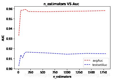
就该数据而言：

• n_estimators=130时，auc指标达到最优
• 后续增加n_estimators，auc提升不明显

max_samples VS auc

maxSamplesNum = []
kFlodsAvgAuc1 = []
testSetAuc1 = []
for i in list(range(10,300,20))+list(range(200,2100,400)):
    print("------- 参数maxSamples=",str(i))
    iForestModel = IsolationForest(n_estimators=130,max_samples=i,n_jobs=-1,random_state=123,verbose=0)
    result = iForestTest(model=iForestModel, kFoldsList=kFoldsList,X_traintotal=X_traintotal,X_test=X_test,y_test=y_test)
    maxSamplesNum.append(i)
    kFlodsAvgAuc1.append(result[0])
    testSetAuc1.append(result[1])

------- 参数maxSamples= 10
------- 参数maxSamples= 30
------- 参数maxSamples= 50
------- 参数maxSamples= 70
------- 参数maxSamples= 90
------- 参数maxSamples= 110
------- 参数maxSamples= 130
------- 参数maxSamples= 150
------- 参数maxSamples= 170
------- 参数maxSamples= 190
------- 参数maxSamples= 210
------- 参数maxSamples= 230
------- 参数maxSamples= 250
------- 参数maxSamples= 270
------- 参数maxSamples= 290
------- 参数maxSamples= 200
------- 参数maxSamples= 600
------- 参数maxSamples= 1000
------- 参数maxSamples= 1400
------- 参数maxSamples= 1800

df2 = pd.DataFrame({"maxSamplesNum":maxSamplesNum,"kFlodsAvgAuc":kFlodsAvgAuc1,"testSetAuc":testSetAuc1})

df2

	maxSamplesNum	kFlodsAvgAuc	testSetAuc
0	10	0.949487	0.903520
1	30	0.951984	0.906453
2	50	0.953766	0.908032
3	70	0.958786	0.909094
4	90	0.959577	0.914187
5	110	0.957167	0.912080
6	130	0.959681	0.911190
7	150	0.958994	0.913248
8	170	0.959381	0.915583
9	190	0.959911	0.914841
10	210	0.958282	0.914825
11	230	0.958917	0.912698
12	250	0.959981	0.916094
13	270	0.960119	0.915770
14	290	0.960576	0.914974
15	200	0.958839	0.914398
16	600	0.959962	0.919391
17	1000	0.960982	0.917315
18	1400	0.961815	0.917679
19	1800	0.960359	0.916489

plt.plot(df2.maxSamplesNum,df2.kFlodsAvgAuc,'r--',label='avgAuc')
plt.plot(df2.maxSamplesNum,df2.testSetAuc,'b--',label='testsetAuc')
plt.title("maxSamples VS Auc  ")
plt.xlabel('maxSamples')
plt.ylabel('AUC')
plt.legend()

contamination对算法效果的影响

contamination和阈值紧密相关，测试不同contamination对precision、recall的影响，方便起见，只观测测试集的效果

y_traintotal.value_counts()

0    227451
1       394
Name: Class, dtype: int64

394/(394+227451)

0.001729245759178389

from sklearn import metrics

for i in [0.0017,0.005,0.01,0.05,0.1]:
    print("---------- contamination: "+str(i))
    iForestModel = IsolationForest(n_estimators=100,max_samples=256,n_jobs=-1,random_state=123,verbose=0,contamination=i)
    iForestModel.fit(X_traintotal)
    test_Pre = iForestModel.predict(X_test)
    test_Pre1 = [1 if i==-1 else 0 for i in list(test_Pre)]
    #--- report
    print('\n',metrics.classification_report(y_test, test_Pre1))    

---------- contamination: 0.0017

               precision    recall  f1-score   support

           0       1.00      1.00      1.00     56864
           1       0.36      0.31      0.33        98

    accuracy                           1.00     56962
   macro avg       0.68      0.65      0.66     56962
weighted avg       1.00      1.00      1.00     56962

---------- contamination: 0.005

               precision    recall  f1-score   support

           0       1.00      1.00      1.00     56864
           1       0.16      0.45      0.24        98

    accuracy                           0.99     56962
   macro avg       0.58      0.72      0.62     56962
weighted avg       1.00      0.99      1.00     56962

---------- contamination: 0.01

               precision    recall  f1-score   support

           0       1.00      0.99      1.00     56864
           1       0.10      0.56      0.17        98

    accuracy                           0.99     56962
   macro avg       0.55      0.78      0.58     56962
weighted avg       1.00      0.99      0.99     56962

---------- contamination: 0.05

               precision    recall  f1-score   support

           0       1.00      0.95      0.98     56864
           1       0.03      0.76      0.05        98

    accuracy                           0.95     56962
   macro avg       0.51      0.85      0.51     56962
weighted avg       1.00      0.95      0.97     56962

---------- contamination: 0.1

               precision    recall  f1-score   support

           0       1.00      0.90      0.95     56864
           1       0.01      0.82      0.03        98

    accuracy                           0.90     56962
   macro avg       0.51      0.86      0.49     56962
weighted avg       1.00      0.90      0.95     56962

Summary

就这个数据集而言：

• 训练集上LR和iForest表现差不多，测试集上LR较优
• 调参对iForest算法提升有限
• 实际应用时，最好不要根据阈值划分，而是去score top数据做验证，归纳规则再应用到实际业务中

Ref

[1] Sklearn文档 https://scikit-learn.org/stable/modules/generated/sklearn.ensemble.IsolationForest.html
[2] Case1文档 https://scikit-learn.org/stable/auto_examples/ensemble/plot_isolation_forest.html#sphx-glr-auto-examples-ensemble-plot-isolation-forest-py
[3] Case2背景 https://www.kaggle.com/mlg-ulb/creditcardfraud
[4] https://zhuanlan.zhihu.com/p/93779599

                                    2020-01-14 于南京市江宁区九龙湖