2017-06-03 Hierarchical Image Saliency Detection on Extended CSSD

Lin Yao

The learning of " Hierarchical Image Saliency Detection on Extended CSSD" (J. Shi, Q. Yan, Li Xu, and J. Jia, IEEE Transactions on Pattern Analysis and Machine Intelligence, Apr. 2016, pp.717-729)

Background

When objects contain salient small-scale patterns, saliency could generally be misled by their complexity. Aiming to solve this notorious and universal problem, this paper proposes a hierarchical framework, to analyze saliency cues from multiple levels of structure, and then integrate them for the final saliency map through hierarchical inference.

Model

1. Layer Generation

1. To produce the three layers, we first generate an initial over segmentation by the watershed-like method.

Use the Gradient Magnitude as the Segmentation Function, The gradient is high at the borders of the objects and low (mostly) inside the objects. Segment the image to get initial map by using the watershed transform.

Grad=Ix2+Iy2

Where Ix indexes the gradient in the horizontal direction, and Iy indexes the gradient in the vertical direction.

1. 
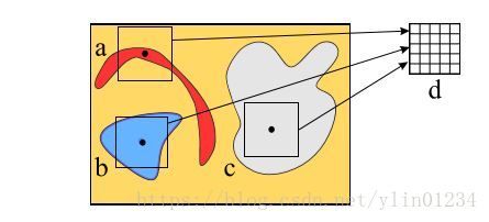
   In fact, a large pixel number does not necessarily correspond to a large-scale region in human perception. This model define a new encompassment scale measure based on shape uniformities and use it to obtain region sizes in the merging process.

scaleR=argmintRt×t|Rt×t⊆R

1. 
   Compute Region Scale

minyDty|y∈Ri>0

Dt=M-kt⋆M , where kt indexes a mean filter of size t×t, and y indexes pixels. It is based on the observation that if all the label values for region Ri in M are altered after the convolution, Ri cannot encompass kt . Thus, the scale of the region is smaller than t.

1. If a region scale is below a selected threshold, merge it to its nearest region, in terms of average CIELUV color distance, and update its scale. In experiment, set thresholds for the three layers as [5, 17, 33.] for typical 400*300 images.

1.  Single-Layer Saliency Cues

1. Local Contrast

Ci=j=1nw(Rj)ϕ(i,j)ci-cj2

Where ci and cj are Lab colors of regions Ri and Rj respectively. wRj counts the number of pixels in Rj. Regions with more pixels contribute higher local-contrast weights than those containing only a few pixels. ϕ(i,j) is set to exp-DRi,Rj/σ2 controlling the spatial distance influence between two regions i and j. Close regions have larger impact than distant ones.

1. Location Heuristic

Hi=1w(Ri)xi∈Riexp-λxi-xc2

Where x0,x1… indexes the set of pixel coordinates in region Ri, and xc is the coordinate of the image center. Hi makes regions close to image center have large weights

1. Saliency value

si'=Ci⋅Hi

Since the local contrast and location cues have been normalized to range [0, 1), their importance is balanced by λ, set to 9 in general. So obtain initial saliency maps separately.

1. Local Consistent Hierarchical Inference

For a node corresponding to region i in layerLk, we define a saliency variable sik. Minimize the following energy function for the hierarchical inference.

Es=kiEDsik+kij,Rik⊆Rjk+1EHsik,sjk+1+kij,Rik∈Α(Rik)ECsik,sjk

The energy consists of three parts.

1. Data term EDsik is to gather separate saliency confidence.

EDsik=βksik-sj-k22

Where βk controls the layer confidence and sj-k is the initial saliency value si'.

1. The hierarchy term EHsik,sjk+1, building cross-layer linkages, enforces consistency between corresponding regions in different layers. A segment is guaranteed to be encompassed by the corresponding ones in upper levels. It not only connects multi-layer information, but also enables reliable combination of saliency results among different scales.

 EHsik,sjk+1=λksik-sjk+122

Where λk controls the strength of consistency between layers. Rik⊆Rjk+1

1. Considering only the influence of corresponding regions in neighboring layers is insufficient. In inference model, we count in a local consistency term between adjacent regions.

The last term is a local consistency term, which enforces intra-layer smoothness. It is used to make saliency assignment smooth between adjacent similar regions.

 ECsik,sjk=γkωi,jksik-sjk22

ωi,jk=exp-cik-cjkσc

Where cik and cjk are mean colors of respective regions.

Energy function including these three terms considers multi-layer saliency cues, making final results have less errors occurred in each single scale.

Optimization

Adopt common loopy belief propagation for optimization. It starts from an initial set of belief propagation messages, and then iterates through each node by applying message passing until convergence.

Iterative formula:

The message passed from region Ri to an adjacent region Rj at the τ times iteration

mi→jτsj=minsiEDsi+ECsi,sj+p∈NRi\jmp→iτ-1(si)

Set NRi contains connected region nodes of Ri, including inter- and intra-layer ones.

If Riand  Rj are regions in different layers

mi→jτsj=minsiEDsi+EHsi,sj+p∈NRi\jmp→iτ-1(si)

After message passing converges atτ times iteration, the optimal value of each saliency variable can be computed via minimizing its belief function.

sj*=minsjEDsj+p∈NRimp→jτ-1(sj)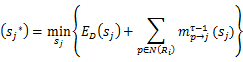

Finally, collect the saliency variables in layer L1 to compute the final saliency map.

Analysis

Proposed method achieves high performance and broadens the feasibility to apply saliency detection to more applications handling different natural images. To a certain extent, it has some effects on the foreground and the background clutter. But still cannot get good results in similar foreground and the background. Moreover, when the region is merged, the threshold value is too large, and a large amount of information loss is easy to occur.