【算法分析】多个对比算法的统计检验方法

一、几种检验方法

先说结论：方差分析（或者用Kruskal Wallis）、秩和检验、Holm's method一定要做。

第一个用于确定所有算法有显著差异，第二个生成p-value用于对比，最后一个用于矫正临界值alpha。

如此对比结果才有说服力。

（1）方差分析（Analysis Of Variance，ANOVA）——推荐1

用于多组样本比较，方差齐，正态性。

（在两组和多组比较中，方差齐性的意思是比较各组的方差大小，看看各组的方差是不是差不多大小，如果差别太大，就认为是方差不齐，或方差不等。）

（2）T检验（T-test）

方差齐，正态性。不齐用矫正T检验。

详见：Python统计分析：[1]独立样本T检验

（3）秩和检验（ Wilcoxon rank sum test）——推荐2

非参数检验。不满足上面做这个。

排秩中的秩是什么？

答：按照变量“数学”中的数据大小进行排秩的，数据最小的排为1，然后以此类推。重复的数据秩次一样，秩次大小为排秩的平均值。比如有2个64，排在第4、5位，平均秩就为4.5。

（4）邦费罗尼校正（Bonferroni Correction）

多重假设的检验中使用的多种p值校正方法的一种保守方法，容易错误地接受零假设。

（5）霍尔姆方法（Holm’s Sequential Bonferroni Procedure，Holm’s method）——推荐3

邦费罗尼校正的一种矫正版本，没有邦费罗尼校正那么严格的条件。更容易发现显著差异，计算难度和邦费罗尼校正一样。

 

---

二、Holm's method详解

 

计算Holm-Bonferroni的公式是：

Where:

• Target alpha level = overall alpha level (usually .05),
• n = number of tests.

计算过程为：（参考链接）

Question: Use the Holm-Bonferroni method to test the following four hypotheses and their associated p-values at an alpha level of .05:  

• H1 = 0.01.
• H2 = 0.04
• H3 = 0.03
• H4 = 0.005

Note: we already know the p-values associated with each hypothesis. If you don’t know the p-values, run a test for each hypothesis before attempting to adjust FWER using the Holm-Bonferroni method. （使用之前，先计算p值）

Step 1: Order the p-values from smallest to greatest:  （p值从小到大排序）

• H4 = 0.005
• H1 = 0.01
• H3 = 0.03
• H2 = 0.04

Step 2: Work the Holm-Bonferroni formula for the first rank: （对第一个rank运行Holm-Bonferroni公式）
HB = Target α / (n – rank + 1)
HB = .05 / (4 – 1 + 1) = .05 / 4 = .0125.

Step 3: Compare the first-ranked (smallest) p-value from Step 1 to the alpha level calculated in Step 2:
Smallest p-value, in Step 1 (H4 = 0.005) < Alpha level in Step 2 (.0125).
If the p-value is smaller, reject the null hypothesis for this individual test.  (p值小于alpha，表明有显著差异)

The p-value of .005 is less than .0125, so the null hypothesis for H4 is rejected.  （第一步的最小p值和第二步的alpha值比较，前者小于后者，则拒绝空假设）

Step 4: Repeat the HB formula for the second rank .  （重复上述步骤给第二个rank）
HB = Target α / (n – rank + 1)
HB = .05 / (4 – 2 + 1) = .05 / 3 = .0167

Step 5: Compare the result from the HB formula in Step 4 to the second-ranked p-value:  
Second ranked p-value, in Step 1 (H1 = 0.01) < Alpha level in Step 2 (.0167).
The p-value of .01 is less than .0167, so the null hypothesis for H1 is rejected as well.

Step 6: Repeat the HB formula for the third rank.（重复上述步骤给第三个rank）
HB = Target α / (n – rank + 1)
HB = .05 / (4 – 3 + 1) = .05 / 2 = .025

Step 7: Compare the result from the HB formula in Step 6 to the third-ranked p-value: 
Third ranked p-value, in Step 1 (H3 = 0.03) > Alpha level in Step 6 (.025).
The p-value of .03 is greater than .025, so the null hypothesis for H3 is not rejected.

The testing stops when you reach the first non-rejected hypothesis. All subsequent hypotheses are non-significant (i.e. not rejected).   （当找到第一个不拒绝的假设时，步骤终止；所有后续假设失效）

Reference:
Holm, S. 1979. A simple sequential rejective multiple test procedure. Scandinavian Journal of Statistics 6:65-70

python代码：

# -*- coding: utf-8 -*-
  
# Import standard packages
import numpy as np
from scipy import stats
import pandas as pd
import os
  
# Other required packages
from statsmodels.stats.multicomp import (pairwise_tukeyhsd,
                                         MultiComparison)
from statsmodels.formula.api import ols
from statsmodels.stats.anova import anova_lm
 
  
#数据excel名              
excel="sample.xlsx"
#读取数据
df=pd.read_excel(excel)
#获取第一组数据，结构为列表
group_mental=list(df.StressReduction[(df.Treatment=="mental")])
group_physical=list(df.StressReduction[(df.Treatment=="physical")])
group_medical=list(df.StressReduction[(df.Treatment=="medical")])
 
 
 
multiComp = MultiComparison(df['StressReduction'], df['Treatment'])
 
def Holm_Bonferroni(multiComp):
    ''' Instead of the Tukey's test, we can do pairwise t-test
    通过均分a=0.05,矫正a,得到更小a'''
      
    # First, with the "Holm" correction
    rtp = multiComp.allpairtest(stats.ttest_rel, method='Holm')
    print((rtp[0]))
      
    # and then with the Bonferroni correction
    print((multiComp.allpairtest(stats.ttest_rel, method='b')[0]))
      
    # Any value, for testing the program for correct execution
    checkVal = rtp[1][0][0,0]
    return checkVal

Holm_Bonferroni(multiComp)

代码来自:https://www.cnblogs.com/webRobot/p/6912257.html , （作者：python_education)

---

三、补充知识

 

1. M个算法，每个运行N次得到数据集怎么称呼？

microarray data，微阵列数据。每个算法运行N次运行结果为一行（或一列）。

gene list，基因列表。每条基因是一个算法运行N次的结果。

2. 为什么要用Holm’s method？

详见 多重检验中p-value的校正

Multiple testing corrections adjust p-values derived from multiple statistical tests to correct for occurrence of false positives. In microarray data analysis, false positives are genes that are found to be statistically different between conditions, but are not in reality.

以Bonferroni correction 为例：

The p-value of each gene is multiplied by the number of genes in the gene list （一个算法重复运行多次得到的一组数据叫做一个基因，每次运行得到基因上的一个基因项）. If the
corrected p-value is still below the error rate, the gene will be significant:
Corrected P-value= p-value * n (number of genes in test) <0.05
As a consequence, if testing 1000 genes at a time, the highest accepted individual pvalue
is 0.00005, making the correction very stringent. With a Family-wise error rate
of 0.05 (i.e., the probability of at least one error in the family), the expected number
of false positives will be 0.05.

3. 为什么p值小于0.05很重要？

详见：https://www.jianshu.com/p/4c9b49878f3d

大部分时候，我们假设错误地拒绝H0的概率为0.05，所以如果p值小于0.05，说明错误地拒绝H0的概率很低，则我们有理由相信H0本身是错误的，而非检验错误导致。
大部分时候p-value用于检验独立变量与输入变量的关系，H0假设通常为假设两者没有关系，所以若p值小于0.05，则可以推翻H0（两者没有关系），推出H1（两者有关系）。

例如: 不同的供应区域是否会对商品单价产生统计显著效果？我们做如下假设：

H0：不同供应区域的商品单价没有差异。（零假设）

H1：不同供应区域的商品单价有显著差异，至少有一个供应区域有不同的商品单价。（非零假设）

如果 p_value > α，我们不能拒绝零假设，表明不同供应区域之间的单价并没有显著差异。

代码表示如下：

if p<0.05:
    print('There is a significant difference.')
else:
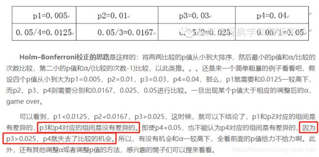
    print('No significant difference.')

另一篇参考文献：http://www.iikx.com/news/statistics/3567.html ，从中可得出，当后续p值被截胡、失去比较机会时，默认是接受空假设，即没有显著差异。