cp9_MathematicalTools_np.linalg.lstsq VS (statsmodels)sm.OLS

import numpy as np
import matplotlib.pyplot as plt
%matplotlib inline

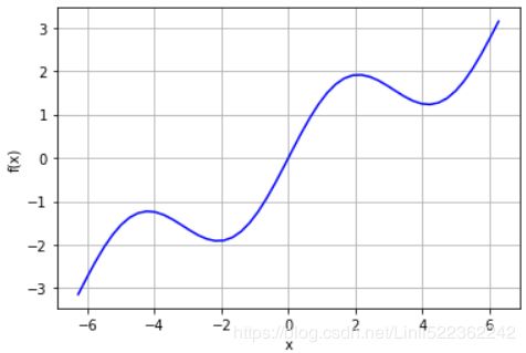
def f(x):
    return np.sin(x) + 0.5 * x

xArr = np.linspace(-2 * np.pi, 2*np.pi, 50)

plt.plot(xArr, f(xArr), 'b')
plt.grid(True)
plt.xlabel('x')
plt.ylabel('f(x)')

#the returned optimal regression coefficients p from polyfit
reg = np.polyfit(xArr, f(xArr), deg=1)
#returns the regression values for the x coordinates
ry = np.polyval(reg, xArr)

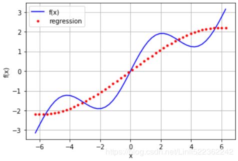
#a linear regression cannot account for the sin part
plt.plot(xArr, f(xArr), 'b', label='f(x)')
plt.plot(xArr, ry, 'r.', label='regression')
plt.legend(loc=0)
plt.grid(True)
plt.xlabel('x')
plt.ylabel('f(x)')

from numpy import polyfit

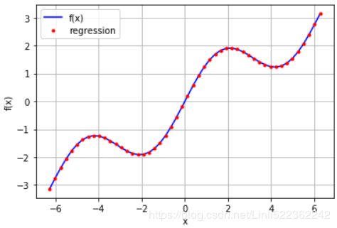
reg = np.polyfit(xArr, f(xArr), deg=5)
ry = np.polyval(reg, xArr)

plt.plot(xArr, f(xArr), 'b', label='f(x)')
plt.plot(xArr, ry, 'r.', label='regression')
plt.legend(loc=0)
plt.grid(True)
plt.xlabel('x')
plt.ylabel('f(x)')

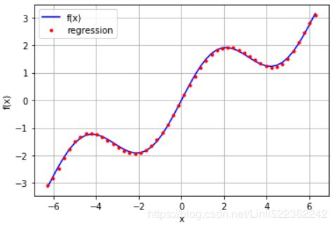
reg = np.polyfit(xArr, f(xArr), deg=7)
ry = np.polyval(reg, xArr)

plt.plot(xArr, f(xArr), 'b', label='f(x)')
plt.plot(xArr, ry, 'r.', label='regression')
plt.legend(loc=0)
plt.grid(True)
plt.xlabel('x')
plt.ylabel('f(x)')

np.allclose(f(xArr), ry)

In general, you can reach better regression results when you can choose better sets of basis
functions, e.g., by exploiting knowledge about the function to approximate. In this case,
the individual basis functions have to be defined via a matrix approach (i.e., using a NumPy
ndarray object). First, the case with monomials up to order 3:

np.sum( (f(xArr)-ry)**2 )/len(xArr)

matrix = np.zeros( (3+1, len(xArr)) )

             #columns: x_vector
matrix[3, :] = xArr**3
matrix[2, :] = xArr**2
matrix[1, :] = xArr
matrix[0, :] = 1
                                
                                               #f(xArr):  single column(f(x)_vector): each row x-- f(x)
reg = np.linalg.lstsq(matrix.T, f(xArr))[0]
ry = np.dot(reg, matrix)

plt.plot(xArr, f(xArr), 'b', label='f(x)')
plt.plot(xArr, ry, 'r.', label = 'regression')
plt.legend(loc=0)
plt.grid(True)
plt.xlabel('x')
plt.ylabel('f(x)')

Using the more general approach allows us to exploit our knowledge about the example function. We know that there is a sin part in the function. Therefore, it makes sense to include a sine function in the set of basis functions.

matrix[3, :] = np.sin(xArr)

reg = np.linalg.lstsq(matrix.T, f(xArr))[0]
ry = np.dot(reg, matrix)

plt.plot(xArr, f(xArr), 'b', label='f(x)')
plt.plot(xArr, ry, 'r.', label='regression')
plt.legend(loc=0)
plt.grid(True)
plt.xlabel('x')
plt.ylabel('f(x)')

np.allclose(f(x), ry)

np.sum((f(x)-ry)**2) / len(x)

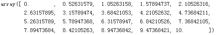
reg #regression coeffeciencies

array([9.26243218e-17, 5.00000000e-01, 0.00000000e+00, 1.00000000e+00])

coefficient

the minimization routine recovers the correct parameters of 1 for the sin part(1.00000000e+00 * sin(x) instead of 1* x^3) and 0.5 for the linear part(5.00000000e-01 *x)

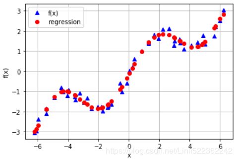
Noisy data

Regression can cope equally well with noisy data, be it data from simulation or from (nonperfect) measurements. To illustrate this point, let us generate both independent observations with noise and also dependent observations with noise:

xn = np.linspace(-2 * np.pi, 2*np.pi, 50)  #Noisy data
xn = xn + 0.15 * np.random.standard_normal(len(xn))
yn = f(xn) + 0.25 * np.random.standard_normal(len(xn))

reg = np.polyfit(xn, yn, 7)
ry = np.polyval(reg, xn)

plt.plot(xn, yn, 'b^', label='f(x)')
plt.plot(xn, ry, 'ro', label='regression')
plt.legend(loc=0)
plt.grid(True)
plt.xlabel('x')
plt.ylabel('f(x)')

Multiple dimension

#def fm((x, y)):
def fm(p):
    x, y = p
    return np.sin(x) + 0.25 * x + np.sqrt(y) + 0.05 * y ** 2

x = np.linspace(0,10,20)
y = np.linspace(0,10,20)
X, Y = np.meshgrid(x,y) #x determines columns; y determines rows 
    #generates 2-d grids out of the 1-d arrays
Z = fm((X,Y))

x = X.flatten() # Yields 1D ndarray objects from the 2D ndarray objects.
y = Y.flatten()
    #yields 1-d arrays from the 2-d grids

np.linspace(0,10,20)

.

a = [[1,3],[2,4],[3,5]]
a = np.array(a) #array([[1, 3],[2, 4],[3, 5]])
a.flatten()     #array([1, 3, 2, 4, 3, 5])

from mpl_toolkits.mplot3d import Axes3D
import matplotlib as mpl

fig = plt.figure(figsize=(9,6))
ax = fig.gca(projection='3d') # get current axis
                               #row_stride           #color-map
surf = ax.plot_surface(X,Y, Z, rstride=2, cstride=2, cmap=mpl.cm.coolwarm, linewidth=0.5, antialiased =True)

ax.set_xlabel=('x')
ax.set_ylabel=('y')
ax.set_zlabel=('f(x,y)')

fig.colorbar(surf, shrink=0.5, aspect=5)

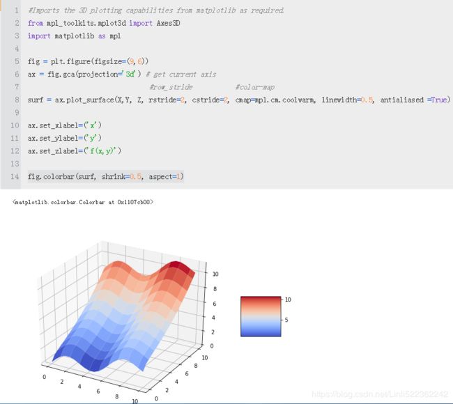
np.sin(x) + 0.25 * x + np.sqrt(y) + 0.05 * y ** 2

#np.sin(x) + 0.25 * x + np.sqrt(y) + 0.05 * y ** 2   #original function
matrix = np.zeros( (len(x), 6+1) )
matrix[:, 6] = np.sqrt(y)
matrix[:, 5] = np.sin(x)
matrix[:, 4] = y ** 2
matrix[:, 3] = x ** 2
matrix[:, 2] = y
matrix[:, 1] = x
matrix[:, 0] = 1

The statsmodels library offers the quite general and helpful function OLS for least-squares regression both in one dimension and multiple dimensions

import statsmodels.api as sm
                #dependent   #variables
model = sm.OLS( fm( (x,y) ), matrix).fit() ###########################

d:\Anaconda3\lib\site-packages\statsmodels\compat\pandas.py:56: FutureWarning: The pandas.core.datetools module is deprecated and will be removed in a future version. Please use the pandas.tseries module instead.
  from pandas.core import datetools

reg = np.linalg.lstsq(matrix, fm((x,y)), rcond=None)[0]

One advantage of using the OLS function is that it provides a wealth of additional information about the regression and its quality. A summary of the results is accessed by calling model.summary. Single statistics, like the coefficient of determination, can in general also be accessed directly:

model.rsquared

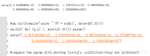
a = model.params #optimal regression parameters,
a

            #coeff  #variables
def reg_func(a, p):
    x,y = p
    f6 = a[6] * np.sqrt(y)
    f5 = a[5] * np.sin(x)
    f4 = a[4] * y**2
    f3 = a[3] * x**2
    f2 = a[2] * y
    f1 = a[1] * x
    f0 = a[0] * 1
    return (f6+f5+f4+f3+f2+f1+f0)

RZ = reg_func(a, (X,Y)) #############

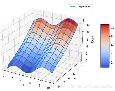
fig = plt.figure(figsize=(9,6))
ax = fig.gca(projection='3d')

surf1 = ax.plot_surface(X,Y,Z, rstride=2, cstride=2,
                       cmap = mpl.cm.coolwarm, linewidth=0.5,
                       antialiased = True)
#wire frame
surf2 = ax.plot_wireframe(X, Y, RZ, rstride=2, cstride=2, label = 'regression')

ax.set_xlabel('x')
ax.set_ylabel('y')
ax.set_zlabel('f(x,y)')
ax.legend()

fig.colorbar(surf1, shrink=0.5, aspect=5)

reg = np.linalg.lstsq(matrix, fm((x, y)), rcond=None)[0]###########################

matrix = np.zeros( (len(x), 6+1) )
matrix[:, 6] = np.sqrt(y)
matrix[:, 5] = np.sin(x)
matrix[:, 4] = y**2
matrix[:, 3] = x**2
matrix[:, 2] = y
matrix[:, 1] = x
matrix[:, 0] = 1

reg = np.linalg.lstsq(matrix, fm((x, y)), rcond=None)[0]###########################
RZZ = np.dot(matrix, reg).reshape( (20, 20) )
# import statsmodels.api as sm
#                 #dependent   #variables
# model = sm.OLS( fm( (x,y) ), matrix).fit() ###########################
# a = model.params 
# RZ = reg_func(a, (X,Y))

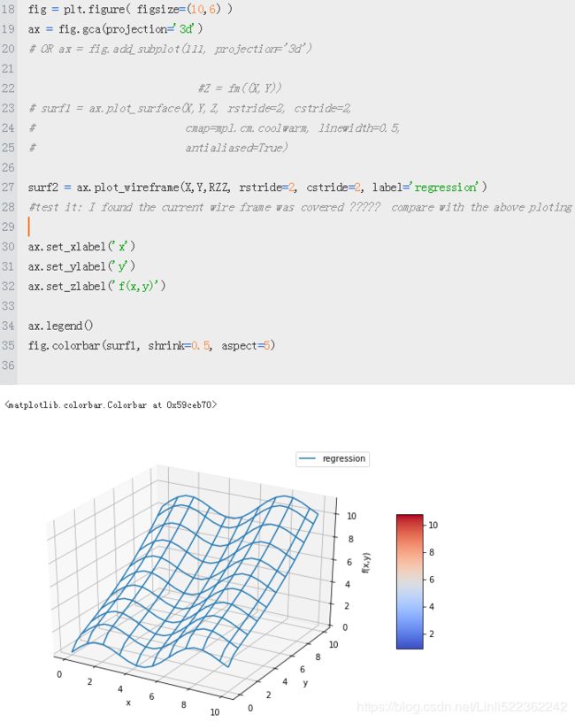
fig = plt.figure( figsize=(10,6) )
ax = fig.gca(projection='3d')
# OR ax = fig.add_subplot(111, projection='3d')

                            #Z = fm((X,Y))
surf1 = ax.plot_surface(X,Y,Z, rstride=2, cstride=2, 
                        cmap=mpl.cm.coolwarm, linewidth=0.5,
                        antialiased=True)

surf2 = ax.plot_wireframe(X,Y,RZZ, rstride=2, cstride=2, label='regression')
#test it: I found the current wire frame was covered ?????  compare with the above ploting

ax.set_xlabel('x')
ax.set_ylabel('y')
ax.set_zlabel('f(x,y)')

ax.legend()
fig.colorbar(surf1, shrink=0.5, aspect=5)

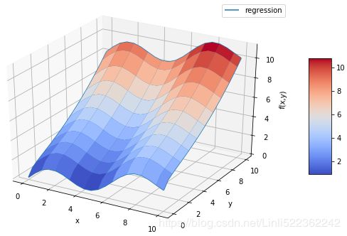
Reason:

matrix = np.zeros( (len(x), 6+1) )
matrix[:, 6] = np.sqrt(y)
matrix[:, 5] = np.sin(x)
matrix[:, 4] = y**2
matrix[:, 3] = x**2
matrix[:, 2] = y
matrix[:, 1] = x
matrix[:, 0] = 1

reg = np.linalg.lstsq(matrix, fm((x, y)), rcond=None)[0]###########################

reg

so

RZZ = np.dot(matrix, reg).reshape( (20, 20) )
# import statsmodels.api as sm
#                 #dependent   #variables
# model = sm.OLS( fm( (x,y) ), matrix).fit() ###########################
# a = model.params 
# RZ = reg_func(a, (X,Y))

fig = plt.figure( figsize=(9,6) )
ax = fig.gca(projection='3d')
# OR ax = fig.add_subplot(111, projection='3d')

                            #Z = fm((X,Y))
surf1 = ax.plot_surface(X,Y,Z, rstride=2, cstride=2, 
                        cmap=mpl.cm.coolwarm, linewidth=0.5,
                        antialiased=True)

surf2 = ax.plot_wireframe(X,Y,RZZ, rstride=2, cstride=2, label='regression')
#test it: I found the current wire frame was covered ?????  compare with the above ploting

ax.set_xlabel('x')
ax.set_ylabel('y')
ax.set_zlabel('f(x,y)')

ax.legend()
fig.colorbar(surf1, shrink=0.5, aspect=5)

Interpolation

Compared to regression, interpolation (e.g., with cubic splines) is more involved mathematically. It is also limited to low-dimensional problems. Given an ordered set of observation points (ordered in the x dimension), the basic idea is to do a regression between two neighboring data points in such a way that not only are the data points perfectly matched by the resulting piecewise-defined interpolation function(分段插值函数), but also the function is continuously differentiable（可微分） at the data points. Continuous differentiability requires at least interpolation of degree 3—i.e., with cubic splines三次样条插值. However, the approach also works in general with quadratic and even linear splines.

splrep函数和splev函数处理回归系数的估计和回归结果的拟合

splrep函数和splev函数处理回归系数的估计和回归结果的拟合

import scipy.interpolate as spi
x = np.linspace(-2 * np.pi, 2*np.pi, 25)

def f(x):
    return np.sin(x) + 0.5*x

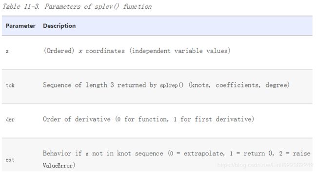
ipo = spi.splrep(x,f(x),k=1) #Sequence of length 3 returned by splrep (knots, coefficients, degree)
iy = spi.splev(x, ipo) #the interpolation already seems really good with linear splines (i.e.,k=1)

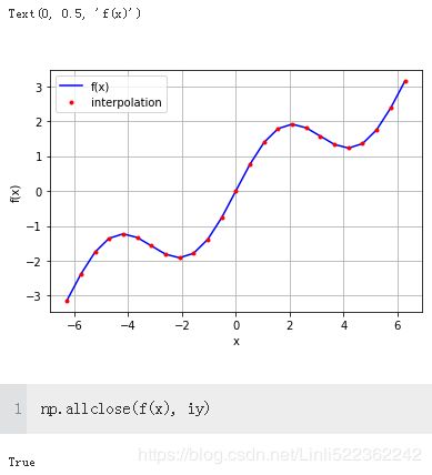
plt.plot(x, f(x), 'b', label='f(x)')
plt.plot(x, iy, 'r.', label='interpolation')

plt.legend(loc=0)
plt.grid(True)
plt.xlabel('x')
plt.ylabel('f(x)')

xd = np.linspace(1.0, 3.0, 50)###a much smaller interval
                    #coeff
iyd = spi.splev(xd, ipo)       #ipo = spi.splrep(x,f(x),k=1) #spline regression plotting

plt.plot(xd, f(xd), 'b', label='f(x)')
plt.plot(xd, iyd, 'r.', label='interpolation')
plt.legend(loc=0)
plt.grid(True)

plt.xlabel('x')
plt.ylabel('y')

ipo = spi.splrep(x, f(x), k=3)  #Sequence of length 3 returned by splrep (knots, coefficients, degree)
iyd = spi.splev(xd, ipo)        #ipo = spi.splrep(x,f(x),k=1)

plt.plot(xd, f(xd),'b', label='f(x)')
plt.plot(xd, iyd, 'r.', label='interpolation')

plt.legend(loc=0)
plt.grid(True)
plt.xlabel('x')
plt.ylabel('f(x)')

INTERPOLATION

In those cases where spline interpolation can be applied you can expect better approximation results compared to a least-squares regression approach. However, remember that you need to have sorted (and “nonnoisy”) data and that the approach is limited to low-dimensional problems. It is also computationally more demanding and might therefore take (much) longer than regression in certain use cases.

Convex Optimization

In finance and economics, convex optimization plays an important role. Examples are the calibration of option pricing models to market data or the optimization of an agent’s utility. As an example function that we want to minimize, we take fm, as defined in the following

def fm(p):
    x,y=p
    return (np.sin(x) + 0.05* x**2 
            + np.sin(y)+0.05* y**2)

x = np.linspace(-10, 10, 50)
y = np.linspace(-10, 10, 50)
X,Y = np.meshgrid(x,y)
Z=fm( (X,Y) )

fig = plt.figure(figsize=(9,6))
ax = fig.gca( projection='3d' )

surf = ax.plot_surface(X,Y,Z, rstride=2, cstride=2, 
                       cmap=mpl.cm.coolwarm, 
                       linewidth=0.5, antialiased =True)
ax.set_xlabel('x')
ax.set_ylabel('y')
ax.set_zlabel('f(x,y)')

fig.colorbar(surf, shrink=0.5, aspect=5)

shows the function graphically for the defined intervals for x and y. Visual inspection already reveals that this function has *multiple local minima. The existence of a global minimum cannot really be confirmed by this particular graphical representation

we want to implement both a global minimization approach and a local one. The functions brute and fmin that we want to use can be found in the sublibrary scipy.optimize:

Global Optimization

To have a closer look behind the scenes when we initiate the minimization procedures, we amend the original function by an option to output current parameter values as well as the function value:

import scipy.optimize as spo
import numpy as np

def fo(p):
    x,y=p
    z = np.sin(x) + 0.05* x**2 + np.sin(y) + 0.05* y**2
    if output ==True:
        print('%8.4f %8.4f %8.4f' % (x,y,z) )
    return z

output=True
               #-10, -5, 0, 5, 10
spo.brute(fo, ((-10,10.1, 5), (-10, 10.1, 5)), finish = None)

output = False
opt1 = spo.brute(fo, ((-10,10.1,0.1), (-10,10.1,0.1)), finish = None)
opt1

def fm(p):
    x,y=p
    return (np.sin(x) + 0.05* x**2 
            + np.sin(y)+0.05* y**2)

fm(opt1)

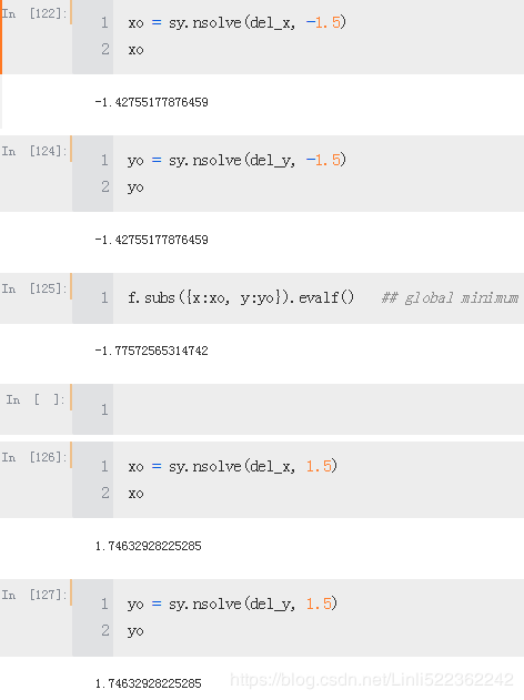
The optimal parameter values are now x = y = –1.4 and the minimal function value for the global minimization is about –1.7749.

Local Optimization

For the local convex optimization we want to draw on the results from the global optimization. The function fmin takes as input the function to minimize and the starting parameter values. In addition, you can define levels for the input parameter tolerance and the function value tolerance, as well as for the maximum number of iterations and function calls:

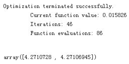
output = True
opt2 = spo.fmin(fo, opt1, xtol=0.001, ftol=0.001, maxiter=15, maxfun=20)
opt2                      ####

array([-1.42702972, -1.42876755]

fm(opt2)

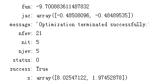
output = False
spo.fmin(fo, (2.0,2.0), maxiter=250)

For many convex optimization problems it is advisable to have a global minimization before the local one. The major reason for this is that local convex optimization algorithms can easily be trapped in a local minimum (or do “basin hopping”), ignoring completely “better” local minima and/or a global minimum. The above shows that setting the starting parameterization to x = y = 2 gives a “minimum” value of above zero

Constrained Optimization

As a simple example, consider the utility maximization problem of an (expected utility maximizing) investor who can invest in two risky securities. Both securities cost qa = qb = 10 today. After one year, they have a payoff of 15 USD and 5 USD, respectively, in state u, and of 5 USD and 12 USD, respectively, in state d. Both states are equally likely. Denote the vector payoffs for the two securities by ra and rb, respectively.

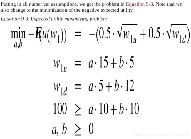
Note(Expected utility maximizing problem) that we also change to the minimization of the negativeexpected utility

# function to be minimized
from math import sqrt

def Eu(p):
    a,b=p
    return -(0.5 * sqrt(a*15 + b*5) + 0.5*sqrt(a*5 + b*12))

# constraints
cons = ({'type': 'ineq', 
         'fun': lambda p: 100-p[0]*10 - p[1]*10 ###############
        })

# budget constraint
bnds = ((0,1000), (0,1000)) #upper bounds large enough

result = spo.minimize(Eu, [5,5], method = 'SLSQP', bounds = bnds, constraints = cons)
result

result['x']  #The optimal parameters

The optimal function value is (changing the sign again):

-result['fun'] #The optimal function value is (changing the sign again):

Given the parameterization for the simple model, it is optimal for the investor to buy about eight unitsof security a and about two units of security b. The budget constraint is binding; i.e., the investor invests his/her total wealth of 100 USD into the securities. This is easily verified through taking the dot product of the optimal parameter vector and the price vector

import numpy as np

np.dot(result['x'],[10,10])

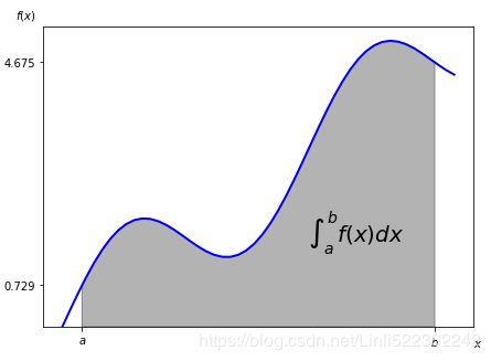
Integration

Especially when it comes to valuation and option pricing, integration is an important mathematical tool. This stems from the fact that risk-neutral values of derivatives can be expressed in general as the discounted expectation of their payoff under the risk-neutral (martingale) measure. The expectation in turn is a sum in the discrete case and an integral in the continuous case. The sublibrary scipy.integrate provides different functions for numerical integration:

import scipy.integrate as sci

def f(x):
    return np.sin(x) + 0.5*x

 

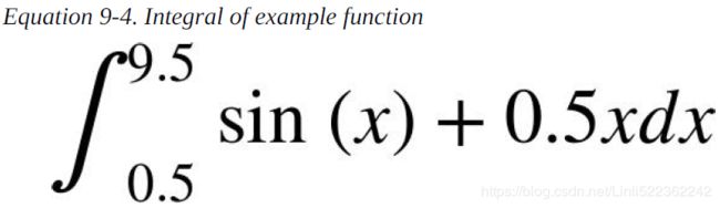
a=0.5 #The integration interval shall be [0.5, 9.5]
b=9.5
x=np.linspace(0,10)
y=f(x)

from matplotlib.patches import Polygon

fig, ax = plt.subplots(figsize=(7,5))
plt.plot(x,y,'b', linewidth=2) #curve
plt.ylim(ymin=0)

#area under the function
#between lower and uppper limit
Ix = np.linspace(a,b)
Iy = f(Ix)
verts = [(a,0)] + list(zip(Ix, Iy)) + [(b,0)]
poly = Polygon(verts, facecolor='0.7', edgecolor='0.5')
ax.add_patch(poly)

#labels
plt.text(0.75 * (a+b), 1.5, r"$\int_a^b f(x)dx$", horizontalalignment="center", fontsize=20)

plt.figtext(0.9, 0.075, '$x$')
plt.figtext(0.075, 0.9, '$f(x)$')

ax.set_xticks((a,b))
ax.set_xticklabels(('$a$', '$b$'))
ax.set_yticks([f(a), f(b)])

Numerical Integration

The integrate sublibrary contains a selection of functions to numerically integrate a given mathematical function given upper and lower integration limits. Examples are fixed_quad for fixed Gaussian quadrature, quad for adaptive quadrature, and romberg for Romberg integration:

sci.fixed_quad(f, a,b)[0]   #above showdow area

sci.quad(f, a, b)[0]

sci.romberg(f, a,b)

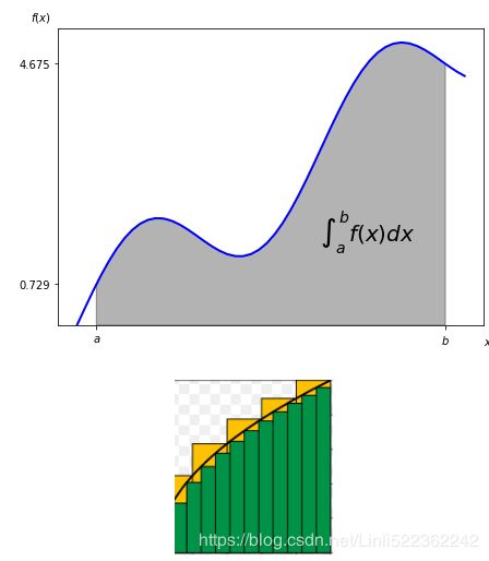
There are also a number of integration functions that take as input list or ndarray objects with function values and input values. Examples in this regard are trapz, using the trapezoidal rule, and simps, implementing Simpson’s rule:

xi = np.linspace(0.5,9.5, 25)
sci.trapz(f(xi), xi)

sci.simps(f(xi), xi)

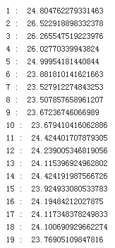
Integration by Simulation

The valuation of options and derivatives by Monte Carlo simulation (cf. Chapter 10) rests on the insight that you can evaluate an integral by simulation. To this end, draw I random values of x between the integral limits[a,b]=[0.5,9.5] and evaluate the integration function at every random value of x. Sum up all the function values and take the average to arrive at an average function value over the integration interval. Multiply this value by the length of the integration interval to derive an estimatefor the integral value.

The following code shows how the Monte Carlo estimated integral value converges to the real one when one increases the number of random draws. The estimator is already quite close for really small numbers of random draws:

for i in range(1,20):
    np.random.seed(1000)
    x=np.random.random(i*10) * (b-a) + a
    print(i,": ",np.sum(f(x))/len(x) *( b-a))

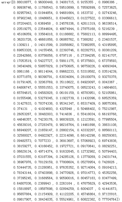
np.random.random(1*10)

array([0.82813023, 0.61078765, 0.28999069, 0.99743849, 0.4192417 ,
       0.89472269, 0.28824616, 0.31344492, 0.98056146, 0.08913687])

np.random.random(19*10)

Symbolic Computation

import sympy as sy

x = sy.Symbol('x')
y = sy.Symbol('y')
type(x)

This already illustrates a major difference. Although x has no numerical value, the square root of x is nevertheless defined with SymPy since x is a Symbol object. In that sense, sy.sqrt(x) can be part of arbitrary mathematical expressions. Notice that SymPy in general automatically simplifies a given mathematical expression

sy.init_printing(pretty_print=False, use_unicode=False)
print(sy.pretty(f))

 

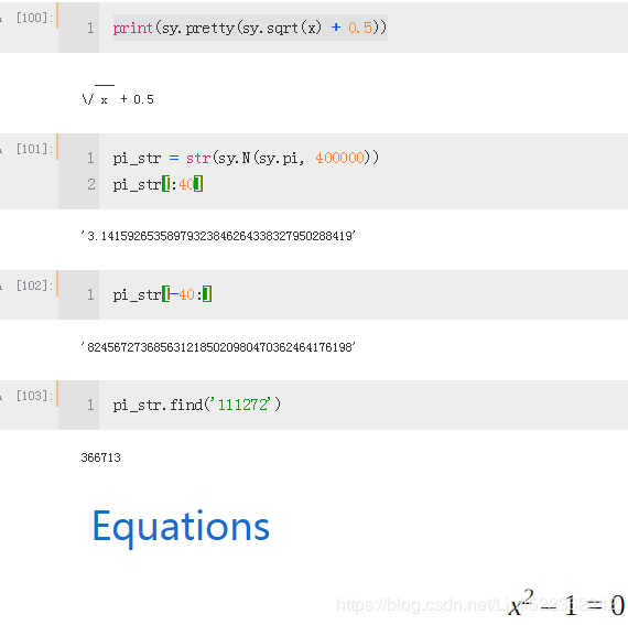
However, there is obviously no guarantee of a solution, either from a mathematical point of view (i.e., the existence of a solution) or from an algorithmic point of view (i.e., an implementation).

Integration

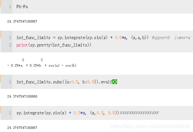
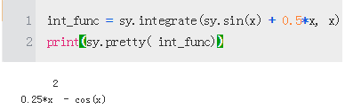
Using integrate, we can then derive the antiderivative of the integration function

int_func = sy.integrate(sy.sin(x) + 0.5*x, x)
print(sy.pretty( int_func))

Fb = int_func.subs(x, 9.5).evalf()
Fa = int_func.subs(x, 0.5).evalf()

Differentiation

The derivative of the antiderivative shall yield in general the original function

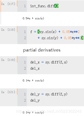
A necessary but not sufficient condition for a global minimum is that both partial derivatives are zero