Supervised Classification——Decision tree

1. 理解

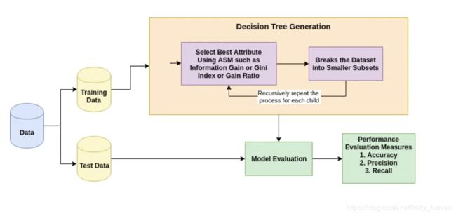
决策树分类算法就是在训练集上建立一个决策树，树的节点是划分树的属性，算法关键就是如何去选择划分的属性。当我们确定好了这个决策树，就可以对测试集的数据进行分类了。

我们需要一个指标(Attribute Selection Measures (ASM))，去评估哪一个属性划分的树更好。常见的指标有Information Gain、Gain Ratio and Gini Index。 这些指标实际上是来源于香农(Shannon)的Information Theory。

Advantages

• Decision trees implicitly perform variable screening or feature selection.
• Decision trees require relatively little effort from users for data preparation.(不需要 standardise/normalise data)
• Nonlinear relationships between parameters do not affect tree performance.
• Can handle both numerical and categorical data. Can also handle multi-output problems. (对于numeric attributes，需要确定breakpoints/Discretisation procedure, 例如：Place breakpoints where the class changes/enforce minimum number of instances in majority class per interval )
• It can be used for feature engineering such as predicting missing values, suitable for variable selection.

Disadvantages

• Decision-tree learners can create over-complex trees that do not generalize the data well. This is called overfitting.
• Sensitive to noisy data.
• Decision trees can be unstable because small variations in the data might result in a completely different tree being generated. This is called variance, which needs to be lowered by methods like bagging and boosting.
• Greedy algorithms cannot guarantee to return the globally optimal decision tree. This can be mitigated by training multiple trees, where the features and samples are randomly sampled with replacement.
• Decision tree learners create biased trees if some classes dominate. It is therefore recommended to balance the data set prior to fitting with the decision tree.

2. 方法

2.1 Attribute Selection Measures

2.1.1 Information Gain

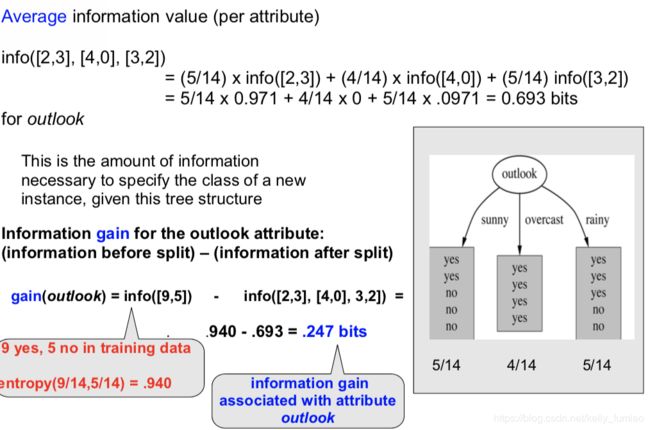
要计算Information Gain， 我们需要知道如何取衡量数据中信息，这里使用的是(shannon) entropy.

$$entropy=-\sum _{i=1}^{n}p(x_i)lo{g}_2(p(x_i))$$
$$info([n_1,n_2,...])=entropy([\frac{n_1}{N},\frac{n_2}{N},...]),N=n_1+n_2+...$$
$$InformationGain=info([beforesplit])-info([aftersplit])$$

Example:

实际上， 我们需要划分之后的entropy最小，而划分前的entropy是固定的，即划分前后的差值要最大，这个差值就是Information Gain。选择产生最大的information gain 属性来划分. 实际上这是一个贪心算法，递归的的split剩下的节点，每一次都选则最好的节点划分。

Information gain computes the difference between entropy before split and average entropy after split of the dataset based on given attribute values.

2.1.2 Gain Ratio

当属性划分之后有很多的分支，Information Gain 会产生比较的偏差。例如， 利用ID来划分，分割ID划分之后每个子分支都只含有一个数据点，此时Info([after split])为0，Information Gain因此也最大。

It means it prefers the attribute with a large number of distinct values. For instance, consider an attribute with a unique identifier such as customer_ID has zero info(D) because of pure partition. This maximizes the information gain and creates useless partitioning.

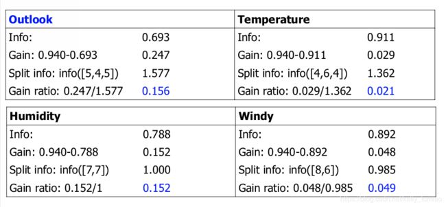
选择属性的时候，Gain ratio 考虑了分支的数量和大小

Gain ratio takes number and size of branches into account when choosing an attribute.

$$GainRatio=<informationgain>/<informationvalueofattribute>$$

Example:

2.1.3 Gini Index

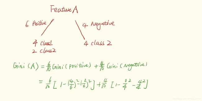
Gini Index表示一个随机选中的样本在子集中被分错的可能性。 K表示分类类别数量。$P_i$表示第 i 类样本的数量占总样本数量的比例。基尼系数的性质与信息熵一样：度量随机变量的不确定度的大小。

• G 越大，数据的不确定性越高；
• G 越小，数据的不确定性越低；
• G = 0，数据集中的所有样本都是同一类别；

$$G=\sum _{i=1}^K{P}_i(1-P_i)=1-\sum _{i=1}^K{P}_i^2，\sum _{i=1}^K{P}_i=1$$

对于样本D,如果根据特征A的某个值a, 把D分成D1和D2两部分，则在特征A的条件下，D的基尼系数表达式为：
$$G(D,A)=\frac{|D_1|}{|D|}Gini(D_1)+\frac{|D_2|}{|D|}Gini(D_2)$$

选择最小的Gini index 的作为划分属性。

Example:

2.2 When to stop splitting

通常来说， 我们可能有许多的features， 这样会使得我们的决策树非常的庞大，而且一直划分的话会有overfitting的问题，所以我们需要 知道什么时候去停止划分树。

• Set a minimum number of training inputs to use on each leaf. For example we can use a minimum of 10 passengers to reach a decision(died or survived), and ignore any leaf that takes less than 10 passengers.
• Set a maximum depth of the decision tree. Maximum depth refers to the the length of the longest path from a root to a leaf.

2.3 Pruning

It involves removing the branches that make use of features having low importance. This way, we reduce the complexity of tree, and thus increasing its predictive power by reducing overfitting.

2.3.1 Post-pruning:

pruning the tree after it has finished

• Minimum error. The tree is pruned back to the point where the cross-validated error is a minimum. Cross-validation is the process of building a tree with most of the data and then using the remaining part of the data to test the accuracy of the decision tree.
• Smallest tree. The tree is pruned back slightly
  further than the minimum error. Technically the pruning creates a decision tree with cross-validation error within 1 standard error of the minimum error. The smaller tree is more intelligible at the cost of a small increase in error.

2.3.2 Pre-pruning/early stopping

stopping the tree before it has completed classifying the training set.

3. 代码

Dataset from kaggle

# Load libraries
import pandas as pd
from sklearn.tree import DecisionTreeClassifier # Import Decision Tree Classifier
from sklearn.model_selection import train_test_split # Import train_test_split function
from sklearn import metrics #Import scikit-learn metrics module for accuracy calculation


# Loading data
col_names = ['pregnant', 'glucose', 'bp', 'skin', 'insulin', 'bmi', 'pedigree', 'age', 'label']
# load dataset
pima = pd.read_csv("pima-indians-diabetes.csv", header=None, names=col_names)
pima.head()

# Feature Selection
#split dataset in features and target variable
feature_cols = ['pregnant', 'insulin', 'bmi', 'age','glucose','bp','pedigree']
X = pima[feature_cols] # Features
y = pima.label # Target variable

# Splitting data
# Split dataset into training set and test set
X_train, X_test, y_train, y_test = train_test_split(X, y, test_size=0.3, random_state=1) # 70% training and 30% test


# Build Decision Tree Model
# Create Decision Tree classifer object
clf = DecisionTreeClassifier()

# Train Decision Tree Classifer
clf = clf.fit(X_train,y_train)

#Predict the response for test dataset
y_pred = clf.predict(X_test)


# Evaluateing Model
# Model Accuracy, how often is the classifier correct?
print("Accuracy:",metrics.accuracy_score(y_test, y_pred))

# Visualizing Decision trees
# pip install graphviz
# pip install pydotplus
from sklearn.tree import export_graphviz
from sklearn.externals.six import StringIO  
from IPython.display import Image  
import pydotplus

dot_data = StringIO()
export_graphviz(clf, out_file=dot_data,  
                filled=True, rounded=True,
                special_characters=True,feature_names = feature_cols,class_names=['0','1'])
graph = pydotplus.graph_from_dot_data(dot_data.getvalue())  
graph.write_png('diabetes.png')
Image(graph.create_png())

优化决策树性能：
clf = DecisionTreeClassifier(criterion = "entropy", max_depth = 3)

• criterion: optional (default=”gini”) or Choose attribute selection measure: This parameter allows us to use the different-different attribute selection measure. Supported criteria are “gini” for the Gini index and “entropy” for the information gain.

• splitter : string, optional (default=”best”) or Split Strategy: This parameter allows us to choose the split strategy. Supported strategies are “best” to choose the best split and “random” to choose the best random split.

• max_depth: int or None, optional (default=None) or Maximum Depth of a Tree: The maximum depth of the tree. If None, then nodes are expanded until all the leaves contain less than min_samples_split samples. The higher value of maximum depth causes overfitting, and a lower value causes underfitting (Source).

• max_leaf_nodes: Reduce the number of leaf nodes

• min_samples_leaf: Restrict the size of sample leaf
  Minimum sample size in terminal nodes can be fixed to 30, 100, 300 or 5% of total

参考

1. Decision Trees in Machine Learning
2. Decision Tree Classification in Python