图像语义分割-----SegNet学习笔记+tensorflow

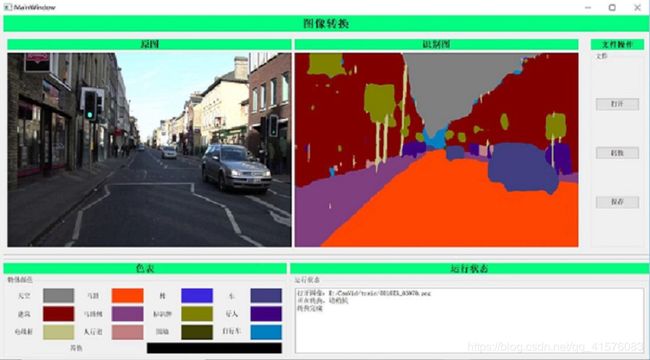
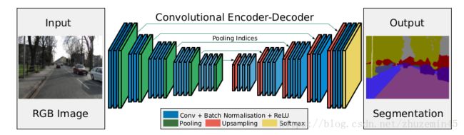
SegNet网络是一个像素级的语义分割模型，即会针对图像中的每一个像素，对每一个像素进行分类，去识别该像素属于的类别，整个网络分为4层下采样以及4层上采样，最后将一个[W, H, 3]的输入图像处理成[W, H, NUM_CLASSES]的向量，再通过softmax进行分类，转化为[W, H, 1]的张量，再对属于不同种类的像素分别涂上不同的颜色，从新变成[W, H, 3]的图像，但是其中的物体以不同的颜色进行了标记区分，这就是SegNet网络的功能：

代码地址：https://github.com/tkuanlun350/Tensorflow-SegNet

代码在model.py中完成了模型搭建，loss定义，以及训练方法，下面就分块记录其实现方式。

一、模型搭建

网络模型并不是很复杂，作者在搭建时将其分为了三个部分，由下向上依次是封装带L2正则化的变量定义，封装带bn层的卷积层与反卷积层定义，封装整个网络，下面也是分开来看：

1.1 变量声明封装

变量声明中又分为向量式变量与矩阵式变量，分别在Utils.py中定义如下：

# 很简单的直接初始化一个shape型向量
def _variable_on_cpu(name, shape, initializer):
  with tf.device('/cpu:0'):
    var = tf.get_variable(name, shape, initializer=initializer)
  return var

# 初始化一个带L2正则化的矩阵变量
def _variable_with_weight_decay(name, shape, initializer, wd):
  # 先初始化一个shape型矩阵变量
  var = _variable_on_cpu(
      name,
      shape,
      initializer)
  # 再根据权重，附加L2正则化并将其正则化loss加入总loss中
  if wd is not None:
    weight_decay = tf.multiply(tf.nn.l2_loss(var), wd, name='weight_loss')
    tf.add_to_collection('losses', weight_decay)
  return var

1.2 卷积层与反卷积层封装

 

卷积层定义：

# 这里作者自己复现了卷积过程，对某一被卷积区域s，通过s*w + b来计算卷积结果
def conv_layer_with_bn(inputT, shape, train_phase, activation=True, name=None):
    # 通过输出通道数目来确定b的维数
    out_channel = shape[3]
    # 初始化卷积核矩阵以及偏移变量
    # 完成卷积计算
    with tf.variable_scope(name) as scope:
      kernel = _variable_with_weight_decay('ort_weights', shape=shape, initializer=orthogonal_initializer(), wd=None)
      conv = tf.nn.conv2d(inputT, kernel, [1, 1, 1, 1], padding='SAME')
      biases = _variable_on_cpu('biases', [out_channel], tf.constant_initializer(0.0))
      bias = tf.nn.bias_add(conv, biases)
      # 通过传入参数中是否使用激活函数标志位
      # 输出bn层输出或者再通过一次relu激活函数
      # bn层定义在下面介绍
      if activation is True:
        conv_out = tf.nn.relu(batch_norm_layer(bias, train_phase, scope.name))
      else:
        conv_out = batch_norm_layer(bias, train_phase, scope.name)
    return conv_out

# bn层在使用时需要确定是否在训练，因为bn层中本身有两个参数是需要训练的
# 非训练模式下，可以直接加载训练后的参数
def batch_norm_layer(inputT, is_training, scope):
  return tf.cond(is_training,
          lambda: tf.contrib.layers.batch_norm(inputT, is_training=True,
                           center=False, updates_collections=None, scope=scope+"_bn"),
          lambda: tf.contrib.layers.batch_norm(inputT, is_training=False,
                           updates_collections=None, center=False, scope=scope+"_bn", reuse = True))

反卷积定义：

def deconv_layer(inputT, f_shape, output_shape, stride=2, name=None):
  strides = [1, stride, stride, 1]
  with tf.variable_scope(name):
    # 首先要用特殊的初始化方式来初始化卷积核，下面给出定义
    weights = get_deconv_filter(f_shape)
    # 进行反卷积操作，这里的反卷积定义可以自行查阅，大概就是先扩充再卷积
    deconv = tf.nn.conv2d_transpose(inputT, weights, output_shape,
                                        strides=strides, padding='SAME')
  return deconv

def get_deconv_filter(f_shape):
  # 此处所用的反卷积核都是2*2的核
  # 其每个位置的参数的初始值由该参数的位置与矩阵尺寸确定，公式如下：
  width = f_shape[0]
  heigh = f_shape[0]
  f = int(width/2.0)
  c = (2 * f - 1 - f % 2) / (2.0 * f)
  bilinear = np.zeros([f_shape[0], f_shape[1]])
  for x in range(width):
      for y in range(heigh):
          value = (1 - abs(x / f - c)) * (1 - abs(y / f - c))
          bilinear[x, y] = value
  weights = np.zeros(f_shape)

  # 由于此处的输入通道与输出通道数目一样，那么就只需要对每个卷积通道上的卷积核进行初始化
  for i in range(f_shape[2]):
      weights[:, :, i, i] = bilinear

  # 利用计算得到的初始值来初始化反卷积核变量
  init = tf.constant_initializer(value=weights,
                                 dtype=tf.float32)
  return tf.get_variable(name="up_filter", initializer=init,
                         shape=weights.shape)

1.3 网络模型搭建

在这里首先要说明一下就是，在整个网络中，一共有八次卷积，4次最大池化以及4次反卷积，其中卷积都是在保持尺寸的模式下进行，而下采样与上采用全部通过池化和反卷积来实现。

def inference(images, labels, batch_size, phase_train):
    # 从conv1到conv4 分别进行4次卷积，以及4次最大池化，得到[batch_num, W/16, H/16, 64]的特征图
    # norm1
    norm1 = tf.nn.lrn(images, depth_radius=5, bias=1.0, alpha=0.0001, beta=0.75,
                name='norm1')
    # conv1
    conv1 = conv_layer_with_bn(norm1, [7, 7, images.get_shape().as_list()[3], 64], phase_train, name="conv1")
    # pool1
    pool1, pool1_indices = tf.nn.max_pool_with_argmax(conv1, ksize=[1, 2, 2, 1], strides=[1, 2, 2, 1],
                           padding='SAME', name='pool1')
    # conv2
    conv2 = conv_layer_with_bn(pool1, [7, 7, 64, 64], phase_train, name="conv2")

    # pool2
    pool2, pool2_indices = tf.nn.max_pool_with_argmax(conv2, ksize=[1, 2, 2, 1],
                           strides=[1, 2, 2, 1], padding='SAME', name='pool2')
    # conv3
    conv3 = conv_layer_with_bn(pool2, [7, 7, 64, 64], phase_train, name="conv3")

    # pool3
    pool3, pool3_indices = tf.nn.max_pool_with_argmax(conv3, ksize=[1, 2, 2, 1],
                           strides=[1, 2, 2, 1], padding='SAME', name='pool3')
    # conv4
    conv4 = conv_layer_with_bn(pool3, [7, 7, 64, 64], phase_train, name="conv4")

    # pool4
    pool4, pool4_indices = tf.nn.max_pool_with_argmax(conv4, ksize=[1, 2, 2, 1],
                           strides=[1, 2, 2, 1], padding='SAME', name='pool4')

    """ End of encoder """
    """ start upsample """
    # upsample4
    # 可选择的针对不同尺寸的输出通过池化操作进行归一化
    # 然后通过upsample4到upsample1进行4次反卷积与卷积操作，得到[batch_num， W， H， 64]的输出
    # upsample4 = upsample_with_pool_indices(pool4, pool4_indices, pool4.get_shape(), out_w=45, out_h=60, scale=2, name='upsample4')
    upsample4 = deconv_layer(pool4, [2, 2, 64, 64], [batch_size, 45, 60, 64], 2, "up4")
    # decode 4
    conv_decode4 = conv_layer_with_bn(upsample4, [7, 7, 64, 64], phase_train, False, name="conv_decode4")

    # upsample 3
    upsample3= deconv_layer(conv_decode4, [2, 2, 64, 64], [batch_size, 90, 120, 64], 2, "up3")
    # decode 3
    conv_decode3 = conv_layer_with_bn(upsample3, [7, 7, 64, 64], phase_train, False, name="conv_decode3")

    # upsample2
    upsample2= deconv_layer(conv_decode3, [2, 2, 64, 64], [batch_size, 180, 240, 64], 2, "up2")
    # decode 2
    conv_decode2 = conv_layer_with_bn(upsample2, [7, 7, 64, 64], phase_train, False, name="conv_decode2")

    # upsample1
    upsample1= deconv_layer(conv_decode2, [2, 2, 64, 64], [batch_size, 360, 480, 64], 2, "up1")
    # decode4
    conv_decode1 = conv_layer_with_bn(upsample1, [7, 7, 64, 64], phase_train, False, name="conv_decode1")
    """ end of Decode """
    """ Start Classify """
    # 通过最后一次卷积操作，得到[batch_num, W, H, NUM_CLASSES]的输出结果作为预测值
    with tf.variable_scope('conv_classifier') as scope:
      # 初始化卷积变量并进行卷积
      kernel = _variable_with_weight_decay('weights',
                                           shape=[1, 1, 64, NUM_CLASSES],
                                           initializer=msra_initializer(1, 64),
                                           wd=0.0005)
      conv = tf.nn.conv2d(conv_decode1, kernel, [1, 1, 1, 1], padding='SAME')
      biases = _variable_on_cpu('biases', [NUM_CLASSES], tf.constant_initializer(0.0))
      conv_classifier = tf.nn.bias_add(conv, biases, name=scope.name)
    # 即为预测值，通过后续的softmax既可以对每一个像素进行分类
    logit = conv_classifier
    # 通过计算logit与labels间的交叉熵来得到loss，当然这里的loss也综合了bn层loss以及L2正则化loss
    loss = cal_loss(conv_classifier, labels)

    return loss, logit

二、loss定义

这里可以这样理解segnet：针对一副图片，假如其有100个像素，那么segnet的功能就是对这幅图片的100个像素，进行100次分类，由于类别信息以one-hot的形式给出，所以loss就是预测值与真值间的交叉熵。

def cal_loss(logits, labels):
    # 考虑到大目标占的像素多，其交叉熵和也较大，因此对应不同物体设定不同的权重
    # 其中面积大的目标权重小，而小物体的权重则要大一些
    loss_weight = np.array([
      0.2595,
      0.1826,
      4.5640,
      0.1417,
      0.9051,
      0.3826,
      9.6446,
      1.8418,
      0.6823,
      6.2478,
      7.3614,
      1.0974]) # class 0~11

    labels = tf.cast(labels, tf.int32)
    # return loss(logits, labels)
    # 通过weigted_loss计算交叉熵以及统计总loss，下面给出其定义
    return weighted_loss(logits, labels, num_classes=NUM_CLASSES, head=loss_weight)

def weighted_loss(logits, labels, num_classes, head=None):
    """ median-frequency re-weighting """
    with tf.name_scope('loss'):

        # 首先把logits整理成[batch_num*W*H, num_classes]格式，分别后续计算
        logits = tf.reshape(logits, (-1, num_classes))

        # epsilon的作用就是防止0的出现，因为log0是无穷，肯定不可以让他出现
        epsilon = tf.constant(value=1e-10)

        # 对预测值都加上epsilon来防止0的出现
        logits = logits + epsilon

        # consturct one-hot label array
        # 下面的两步将类别标签也整理成[batch_num*W*H, num_classes]格式
        label_flat = tf.reshape(labels, (-1, 1))
        # should be [batch ,num_classes]
        labels = tf.reshape(tf.one_hot(label_flat, depth=num_classes), (-1, num_classes))

        # 对预测值进行softmax
        softmax = tf.nn.softmax(logits)

        # 下面的两步就是一个带权重的交叉熵计算
        cross_entropy = -tf.reduce_sum(tf.multiply(labels * tf.log(softmax + epsilon), head), axis=[1])

        cross_entropy_mean = tf.reduce_mean(cross_entropy, name='cross_entropy')

        # 将预测loss加入总的loss
        tf.add_to_collection('losses', cross_entropy_mean)
        # 提取全部loss，这里就包含了L2正则化loss以及bn层loss
        loss = tf.add_n(tf.get_collection('losses'), name='total_loss')

    return loss

三、训练方法

首先来看一下优化器的定义

def train(total_loss, global_step):
    total_sample = 274
    num_batches_per_epoch = 274/1
    """ fix lr """
    lr = INITIAL_LEARNING_RATE
    loss_averages_op = _add_loss_summaries(total_loss)

    # Compute gradients.
    # 在计算梯度应用梯度前，先做一步loss收集，这里仅供记录用
    with tf.control_dependencies([loss_averages_op]):
      # 调用确定学习率lr的adam优化器
      opt = tf.train.AdamOptimizer(lr)
      # 根据当前loss计算优化梯度
      grads = opt.compute_gradients(total_loss)
    # 将优化梯度应用至各个变量上，注意apply_gradients也是自带使global_step自动加一的功能
    apply_gradient_op = opt.apply_gradients(grads, global_step=global_step)

    # Add histograms for trainable variables.
    for var in tf.trainable_variables():
      tf.summary.histogram(var.op.name, var)

    # Add histograms for gradients.
    for grad, var in grads:
      if grad is not None:
        tf.summary.histogram(var.op.name + '/gradients', grad)

    # Track the moving averages of all trainable variables.
    variable_averages = tf.train.ExponentialMovingAverage(
        MOVING_AVERAGE_DECAY, global_step)
    variables_averages_op = variable_averages.apply(tf.trainable_variables())

    # 这里看到运行train_op之前就会先计算loss梯度并优化和计算滑动平均
    # 所以针对一次训练，传入样本和标签后，run一次train_op就是训练了一步
    with tf.control_dependencies([apply_gradient_op, variables_averages_op]):
      train_op = tf.no_op(name='train')

    return train_op

然后看一下样本是如何加载的，这里大概说一下，样本由三部分组成，一个txt和两个文件夹，txt中每一行按顺序放的是原图和类别图地址，另外两个文件夹中就是放的对应的图片，类别图就是每一个像素的值，都是原图中对应位置像素的类别代号（比如自行车是10，那类别图对应原图直行车的地方就全是像素10）

样本的加载函数都在Inputs.py中得到实现，代码很简单易懂，就是读txt中每行的两个路径，再分别读出来其图片，作为images和labels，再通过使用tf.train.batch（）函数来生成每一个batch，这里就不在累述。

直接看training函数：

def training(FLAGS, is_finetune=False):
  # 下面的都是一些设置系数，其中几个地址就是样本集的存放地址，可以看情况来更改
  max_steps = FLAGS.max_steps
  batch_size = FLAGS.batch_size
  train_dir = FLAGS.log_dir # /tmp3/first350/TensorFlow/Logs
  image_dir = FLAGS.image_dir # /tmp3/first350/SegNet-Tutorial/CamVid/train.txt
  val_dir = FLAGS.val_dir # /tmp3/first350/SegNet-Tutorial/CamVid/val.txt
  finetune_ckpt = FLAGS.finetune
  image_w = FLAGS.image_w
  image_h = FLAGS.image_h
  image_c = FLAGS.image_c
  # should be changed if your model stored by different convention
  startstep = 0 if not is_finetune else int(FLAGS.finetune.split('-')[-1])

  # 先成对读取样本与标签的地址
  # 其中val开头的是测试集
  image_filenames, label_filenames = get_filename_list(image_dir)
  val_image_filenames, val_label_filenames = get_filename_list(val_dir)

  with tf.Graph().as_default():
    
    # 在计算图中，设定几个占位符，这也是整个网络需要的输入
    train_data_node = tf.placeholder( tf.float32, shape=[batch_size, image_h, image_w, image_c])

    train_labels_node = tf.placeholder(tf.int64, shape=[batch_size, image_h, image_w, 1])

    phase_train = tf.placeholder(tf.bool, name='phase_train')

    global_step = tf.Variable(0, trainable=False)

    # 获得一个batch的样本
    images, labels = CamVidInputs(image_filenames, label_filenames, batch_size)

    val_images, val_labels = CamVidInputs(val_image_filenames, val_label_filenames, batch_size)

    # 构建loss与预测值计算节点，并将loss传入train函数构建训练节点train_op
    loss, eval_prediction = inference(train_data_node, train_labels_node, batch_size, phase_train)
    train_op = train(loss, global_step)

    # 根据是否是finetune来加载预训练参数
    saver = tf.train.Saver(tf.global_variables())
    summary_op = tf.summary.merge_all()
    with tf.Session() as sess:
      if (is_finetune == True):
          saver.restore(sess, finetune_ckpt )
      else:
          init = tf.global_variables_initializer()
          sess.run(init)

      # 这里还运用了多线程进行训练，设立了线程池
      coord = tf.train.Coordinator()
      threads = tf.train.start_queue_runners(sess=sess, coord=coord)

      # Summery placeholders
      summary_writer = tf.summary.FileWriter(train_dir, sess.graph)
      average_pl = tf.placeholder(tf.float32)
      acc_pl = tf.placeholder(tf.float32)
      iu_pl = tf.placeholder(tf.float32)
      average_summary = tf.summary.scalar("test_average_loss", average_pl)
      acc_summary = tf.summary.scalar("test_accuracy", acc_pl)
      iu_summary = tf.summary.scalar("Mean_IU", iu_pl)

      # 在这里正式开始训练，可以看到，加载一个batch的样本然后传入，run训练节点train_op即为一次训练
      for step in range(startstep, startstep + max_steps):
        print(step)
        image_batch ,label_batch = sess.run([images, labels])
        feed_dict = {
          train_data_node: image_batch,
          train_labels_node: label_batch,
          phase_train: True
        }
        start_time = time.time()

        _, loss_value = sess.run([train_op, loss], feed_dict=feed_dict)
        duration = time.time() - start_time

        assert not np.isnan(loss_value), 'Model diverged with loss = NaN'

        # 每10步打印一次loss以及在训练集上的准确度
        if step % 10 == 0:
          num_examples_per_step = batch_size
          examples_per_sec = num_examples_per_step / duration
          sec_per_batch = float(duration)

          format_str = ('%s: step %d, loss = %.2f (%.1f examples/sec; %.3f '
                      'sec/batch)')
          print (format_str % (datetime.now(), step, loss_value,
                               examples_per_sec, sec_per_batch))

          # eval current training batch pre-class accuracy
          pred = sess.run(eval_prediction, feed_dict=feed_dict)
          per_class_acc(pred, label_batch)
        
        # 每100步打印loss及在测试集上的准确度
        if step % 100 == 0:
          print("start validating.....")
          total_val_loss = 0.0
          hist = np.zeros((NUM_CLASSES, NUM_CLASSES))
          for test_step in range(int(TEST_ITER)):
            val_images_batch, val_labels_batch = sess.run([val_images, val_labels])

            _val_loss, _val_pred = sess.run([loss, eval_prediction], feed_dict={
              train_data_node: val_images_batch,
              train_labels_node: val_labels_batch,
              phase_train: True
            })
            total_val_loss += _val_loss
            hist += get_hist(_val_pred, val_labels_batch)
          print("val loss: ", total_val_loss / TEST_ITER)
          acc_total = np.diag(hist).sum() / hist.sum()
          iu = np.diag(hist) / (hist.sum(1) + hist.sum(0) - np.diag(hist))
          test_summary_str = sess.run(average_summary, feed_dict={average_pl: total_val_loss / TEST_ITER})
          acc_summary_str = sess.run(acc_summary, feed_dict={acc_pl: acc_total})
          iu_summary_str = sess.run(iu_summary, feed_dict={iu_pl: np.nanmean(iu)})
          print_hist_summery(hist)
          print(" end validating.... ")

          summary_str = sess.run(summary_op, feed_dict=feed_dict)
          summary_writer.add_summary(summary_str, step)
          summary_writer.add_summary(test_summary_str, step)
          summary_writer.add_summary(acc_summary_str, step)
          summary_writer.add_summary(iu_summary_str, step)
        # Save the model checkpoint periodically.

        # 每1000步存储一次参数
        if step % 1000 == 0 or (step + 1) == max_steps:
          checkpoint_path = os.path.join(train_dir, 'model.ckpt')
          saver.save(sess, checkpoint_path, global_step=step)

      coord.request_stop()
      coord.join(threads)

总体整个segnet还是很好玩的一个网络，生成的图片也很好看，但是不知道是不是这个代码的作者在写writeImage这个函数的时候是不是把顺序写错了，导致检测后的涂色和官网不一样，这里放一下该函数：

# 根据预测的类别代号，涂色，但是这里好像顺序错了，比如Car在这里是第10个，那么其代号就是9，但是官网的结果好像其代号不应该是9
def writeImage(image, filename):
    """ store label data to colored image """
    Sky = [128,128,128]
    Building = [128,0,0]
    Pole = [192,192,128]
    Road_marking = [255,69,0]
    Road = [128,64,128]
    Pavement = [60,40,222]
    Tree = [128,128,0]
    SignSymbol = [192,128,128]
    Fence = [64,64,128]
    Car = [64,0,128]
    Pedestrian = [64,64,0]
    Bicyclist = [0,128,192]
    Unlabelled = [0,0,0]
    r = image.copy()
    g = image.copy()
    b = image.copy()
    label_colours = np.array([Sky, Building, Pole, Road_marking, Road, Pavement, Tree, SignSymbol, Fence, Car, Pedestrian, Bicyclist, Unlabelled])
    # 根据每个像素的类别，涂不同的颜色
    for l in range(0,12):
        r[image==l] = label_colours[l,0]
        g[image==l] = label_colours[l,1]
        b[image==l] = label_colours[l,2]
    rgb = np.zeros((image.shape[0], image.shape[1], 3))
    rgb[:,:,0] = r/1.0
    rgb[:,:,1] = g/1.0
    rgb[:,:,2] = b/1.0
    im = Image.fromarray(np.uint8(rgb))
    im.save(filename)

下面是测试图像，我按实际情况改了改颜色，而且自己训练的参数效果还是有缺陷：