机器学习案例实战：Python实现逻辑回归与梯度下降策略

原创文章,如需转载请保留出处
本博客为唐宇迪老师python数据分析与机器学习实战课程学习笔记

一. Python实现逻辑回归任务概述
1.1 问题描述
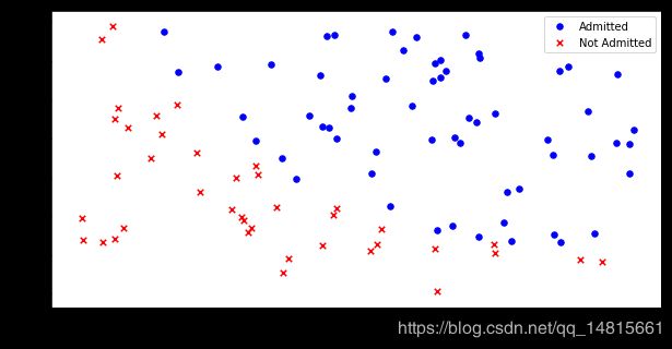
我们将建立一个逻辑回归模型来预测一个学生是否被大学录取。假设你是一个大学系的管理员，你想根据两次考试的结果来决定每个申请人的历史数据，你可以用它作为逻辑回归的训练集。对于每一个培训例子，你可以有两个考试申请人的分数和录取决定。为了做到这一点，我们将建立一个分类模型，根据考试成绩估计入学概率。

1.2 代码实现

import numpy as np
import pandas as pd
import matplotlib.pyplot as plt
%matplotlib inline

import os
path = 'data'+os.sep+'LogiReg_data.txt'
pdData = pd.read_csv(path, header=None, names=['Exam 1','Exam 2','Admitted'])
pdData.head()

Exam 1 Exam 2 Admitted
0 34.623660 78.024693 0
1 30.286711 43.894998 0
2 35.847409 72.902198 0
3 60.182599 86.308552 1
4 79.032736 75.344376 1

pdData.shape

(100, 3)

#fig, ax = plt.subplots(1,3,figsize=(15,7))，这样就会有1行3个15x7大小的子图。
positive = pdData[pdData['Admitted']==1]
negative = pdData[pdData['Admitted']==0]

fig,ax = plt.subplots(figsize=(10,5))
ax.scatter(positive['Exam 1'],positive['Exam 2'],s=30,c='b',marker='o',label='Admitted')
ax.scatter(negative['Exam 1'],negative['Exam 2'],s=30,c='r',marker='x',label='Not Admitted')
ax.legend()
ax.set_xlabel('Exam 1 Score')
ax.set_ylabel('Exam 2 Score')

1.3 The logistic regression

• 目标：建立分类器（求解出三个参数θ0θ1θ2）
• 设定阈值，根据阈值判断录取结果

要完成的模块

• sigmoid：映射到概率的函数
• model：返回预测结果值
• cost：根据参数计算损失
• gradient：计算每个参数的梯度方向
• descent：进行参数更新
• accuracy：计算精度

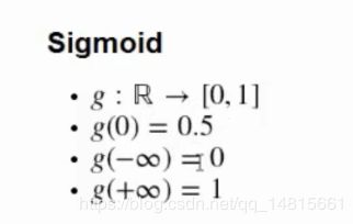
Sigmoid函数

二. 完成梯度下降模块
2.1 Sigmoid函数定义

def sigmoid(z):
    return 1/(1 + np.exp(-z))

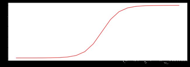
2.2 查看该函数

nums = np.arange(-10, 10, step=1)
fig, ax = plt.subplots(figsize=(12,4))
ax.plot(nums, sigmoid(nums),'r')

2.3 完成model函数定义

def model(X,theta):
    return sigmoid(np.dot(X, theta.T))

2.4 定义参数

pdData.insert(0, 'Ones', 1)
##将表格转换为矩阵
orig_data = pdData.as_matrix()
cols = orig_data.shape[1]#cols=4列
X = orig_data[:,0:cols-1]
y = orig_data[:,cols-1:cols]
theta = np.zeros([1,3])

2.5 查看参数

X[:5]

array([[ 1. , 34.62365962, 78.02469282],
[ 1. , 30.28671077, 43.89499752],
[ 1. , 35.84740877, 72.90219803],
[ 1. , 60.18259939, 86.3085521 ],
[ 1. , 79.03273605, 75.34437644]])

y[:5]

array([[0.],
[0.],
[0.],
[1.],
[1.]])

theta

array([[0., 0., 0.]])

X.shape, y.shape, theta.shape

((100, 3), (100, 1), (1, 3))

2.6 定义损失函数

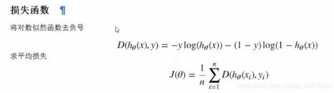
def cost(X, y, theta):
    left = np.multiply(-y, np.log(model(X, theta)))
    right = np.multiply(1 - y, np.log(1-model(X, theta)))
    return np.sum(left - right) / (len(X))

2.7 带入计算

cost(X, y, theta)

0.6931471805599453

2.8 计算梯度
批量梯度下降法：

def gradient(X, y, theta):
    grad = np.zeros(theta.shape)
    error = (model(X, theta) - y).ravel()
    for j in range(len(theta.ravel())):
        term = np.multiply(error, X[:,j])
        grad[0,j] = np.sum(term) / len(X)
    return grad

三. 停止策略与梯度下降案例

STOP_ITER = 0
STOP_COST = 1
STOP_GRAD = 2

def stopCriterion(type, value, threshold):
    #设定三种不同的停止策略
    if type == STOP_ITER:   return value > threshold
    elif type == STOP_COST: return abs(value[-1]-value[-2]) < threshold
    elif type == STOP_GRAD: return np.linalg.norm(value) < threshold

import numpy.random
#洗牌
def shuffleData(data):
    np.random.shuffle(data)
    cols = data.shape[1]
    X = data[:, 0:cols-1]
    y = data[:, cols-1:]
    return X, y

import time

def descent(data, theta, batchSize, stopType, thresh, alpha):
    #梯度下降求解
    init_time = time.time()
    i = 0#迭代次数
    k = 0#batch
    X, y = shuffleData(data)
    grad = np.zeros(theta.shape)#计算的梯度
    costs = [cost(X, y, theta)]#损失值
    
    while True:
        grad = gradient(X[k:k+batchSize], y[k:k+batchSize], theta)
        k += batchSize#取batch数量个数据
        if k>=n:
            k = 0
            X, y = shuffleData(data)#重新洗牌
        theta = theta - alpha*grad#参数更新
        costs.append(cost(X, y, theta))#计算新的损失
        i +=1
        
        if stopType == STOP_ITER:   value = i
        elif stopType == STOP_COST: value = costs
        elif stopType == STOP_GRAD: value = grad
        if stopCriterion(stopType, value, thresh):break
    return theta, i-1, costs, grad, time.time() - init_time

def runExpe(data, theta, batchSize, stopType, thresh, alpha):
    theta, iter, costs, grad, dur = descent(data, theta, batchSize, stopType, thresh, alpha)
    name = "Original" if (data[:,1]>2).sum() > 1 else "Scaled"
    name += "data - learning rate:{} -".format(alpha)
    if batchSize==n:strDescType = "Gradient"
    elif batchSize == 1: strDescType = "Stochastic"
    else: strDescType = "Mini-batch({})".format(batchSize)
    name += strDescType + "descent - Stop:"
    if stopType == STOP_ITER: strStop = "{} iterations".format(thresh)
    elif stopType == STOP_ITER: strStop = "costs change < {}".format(thresh)
    else: strStop ="gradient norm < {}".format(thresh)
    name+=strStop
    print ("***{}\nTheta:{} - Iter:{} - Last cost:{:03.2f} - Duration:{:03.2f}s".format(
        name, theta, iter, costs[-1],dur))
    fig, ax = plt.subplots(figsize=(12,4))
    ax.plot(np.arange(len(costs)),costs,'r')
    ax.set_xlabel('Iterations')
    ax.set_ylabel('Cost')
    ax.set_title(name.upper() + ' - Error vs. Iteration')
    return theta

n = 100
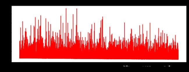
runExpe(orig_data, theta, n, STOP_ITER, thresh=5000, alpha=0.000001)

四. 实验对比效果
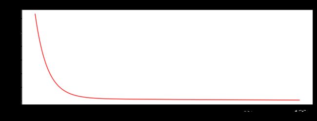
4.1 根据损失值停止
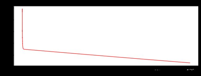
设定阈值1E-6，差不多需要110000次迭代

runExpe(orig_data, theta, n, STOP_COST, thresh=0.000001, alpha=0.001)

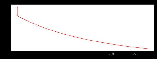
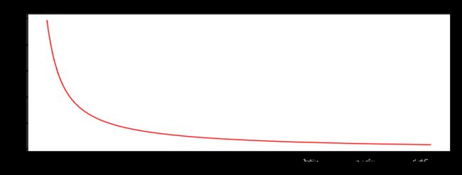
4.2 根据梯度变化停止
设定阈值0.05，差不多需要40000次迭代

runExpe(orig_data, theta, n, STOP_GRAD, thresh=0.05, alpha=0.001)

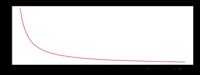
4.3 对比不同的梯度下降方法

runExpe(orig_data, theta, 1, STOP_ITER, thresh=5000, alpha=0.001)

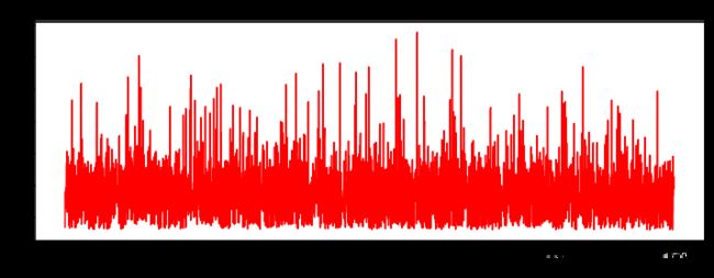
runExpe(orig_data, theta, 1, STOP_ITER, thresh=15000, alpha=0.000002)

runExpe(orig_data, theta, 16, STOP_ITER, thresh=15000, alpha=0.001)

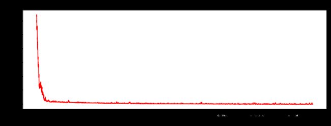
浮动依然比较大，我们尝试对数据标准化，将数据按其属性（按列进行）减去其均值，然后除以其方差。最后得到的结果是，对每个属性/每列来说所有数据都聚集在0附近，方差值为1

from sklearn import preprocessing as pp

scaled_data = orig_data.copy()
scaled_data[:,1:3] = pp.scale(orig_data[:,1:3])

runExpe(orig_data, theta, n, STOP_ITER, thresh=5000, alpha=0.001)

runExpe(orig_data, theta, n, STOP_GRAD, thresh=0.02, alpha=0.001)

runExpe(orig_data, theta, n, STOP_GRAD, thresh=0.02, alpha=0.001)

runExpe(scaled_data, theta, 16, STOP_GRAD, thresh=0.002*2, alpha=0.001)

4.4 精度

#设定阈值
def predict (X, theta):
    return [1 if x >=0.5 else 0 for x in model(X, theta)]

scaled_X = scaled_data[:, :3]
y = scaled_data[:, 3]
predictions = predict(scaled_X, theta)
correct = [1 if ((a == 1 and b == 1) or (a == 0 and b == 0)) else 0 for (a, b) in zip(predictions, y)]
accuracy = (sum(map(int, correct)) % len(correct))
print ('accuracy = {0}%'.format(accuracy))

accuracy = 89%