深度学习-卷积神经网络 吴恩达第四课第二周作业2答案(Residual Networks)

import numpy as np
import tensorflow as tf
from keras import layers
from keras.layers import Input, Add, Dense, Activation, ZeroPadding2D, BatchNormalization, Flatten, Conv2D, AveragePooling2D, MaxPooling2D, GlobalMaxPooling2D
from keras.models import Model, load_model
from keras.preprocessing import image
from keras.utils import layer_utils
from keras.utils.data_utils import get_file
from keras.applications.imagenet_utils import preprocess_input
import pydot
from IPython.display import SVG
from keras.utils.vis_utils import model_to_dot
from keras.utils import plot_model
from resnets_utils import *
from keras.initializers import glorot_uniform
import scipy.misc
from matplotlib.pyplot import imshow
%matplotlib inline

import keras.backend as K
K.set_image_data_format('channels_last')
K.set_learning_phase(1)

# GRADED FUNCTION: identity_block

def identity_block(X, f, filters, stage, block):
    """
    Implementation of the identity block as defined in Figure 4
    
    Arguments:
    X -- input tensor of shape (m, n_H_prev, n_W_prev, n_C_prev)
    f -- integer, specifying the shape of the middle CONV's window for the main path
    filters -- python list of integers, defining the number of filters in the CONV layers of the main path
    stage -- integer, used to name the layers, depending on their position in the network
    block -- string/character, used to name the layers, depending on their position in the network
    
    Returns:
    X -- output of the identity block, tensor of shape (n_H, n_W, n_C)
    """
    
    # defining name basis
    conv_name_base = 'res' + str(stage) + block + '_branch'
    bn_name_base = 'bn' + str(stage) + block + '_branch'
    
    # Retrieve Filters
    F1, F2, F3 = filters
    
    # Save the input value. You'll need this later to add back to the main path. 
    X_shortcut = X
    
    # First component of main path
    X = Conv2D(filters = F1, kernel_size = (1, 1), strides = (1,1), padding = 'valid', name = conv_name_base + '2a', kernel_initializer = glorot_uniform(seed=0))(X)
    X = BatchNormalization(axis = 3, name = bn_name_base + '2a')(X)
    X = Activation('relu')(X)
    
    ### START CODE HERE ###
    
    # Second component of main path (≈3 lines)
    X = Conv2D(filters=F2, kernel_size=(f, f), strides=(1,1), padding='same', name = conv_name_base+'2b', kernel_initializer=glorot_uniform(seed=0))(X)
    X = BatchNormalization(axis=3, name=bn_name_base+'2b')(X)
    X = Activation('relu')(X)

    # Third component of main path (≈2 lines)
    X = Conv2D(filters=F3, kernel_size=(1, 1), strides=(1,1), padding='valid', name = conv_name_base+'2c', kernel_initializer=glorot_uniform(seed=0))(X)
    X = BatchNormalization(axis=3, name=bn_name_base+'2c')(X)

    # Final step: Add shortcut value to main path, and pass it through a RELU activation (≈2 lines)
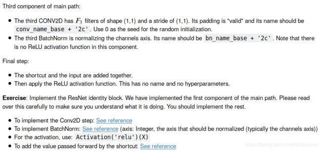
    X = Add()([X, X_shortcut])
    X = Activation('relu')(X)
    
    ### END CODE HERE ###
    
    return X

tf.reset_default_graph()

with tf.Session() as test:
    np.random.seed(1)
    A_prev = tf.placeholder("float", [3, 4, 4, 6])
    X = np.random.randn(3, 4, 4, 6)
    A = identity_block(A_prev, f = 2, filters = [2, 4, 6], stage = 1, block = 'a')
    test.run(tf.global_variables_initializer())
    out = test.run([A], feed_dict={A_prev: X, K.learning_phase(): 0})
    print("out = " + str(out[0][1][1][0]))

out = [0.19716814 0.         1.3561226  2.1713073  0.         1.3324987 ]

# GRADED FUNCTION: convolutional_block

def convolutional_block(X, f, filters, stage, block, s = 2):
    """
    Implementation of the convolutional block as defined in Figure 4
    
    Arguments:
    X -- input tensor of shape (m, n_H_prev, n_W_prev, n_C_prev)
    f -- integer, specifying the shape of the middle CONV's window for the main path
    filters -- python list of integers, defining the number of filters in the CONV layers of the main path
    stage -- integer, used to name the layers, depending on their position in the network
    block -- string/character, used to name the layers, depending on their position in the network
    s -- Integer, specifying the stride to be used
    
    Returns:
    X -- output of the convolutional block, tensor of shape (n_H, n_W, n_C)
    """
    
    # defining name basis
    conv_name_base = 'res' + str(stage) + block + '_branch'
    bn_name_base = 'bn' + str(stage) + block + '_branch'
    
    # Retrieve Filters
    F1, F2, F3 = filters
    
    # Save the input value
    X_shortcut = X


    ##### MAIN PATH #####
    # First component of main path 
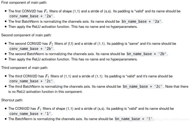
    X = Conv2D(filters=F1, kernel_size=(1,1), strides=(s,s), \
               padding='valid', name = conv_name_base+'2a', kernel_initializer=glorot_uniform(seed=0))(X)
    X = BatchNormalization(axis=3, name=bn_name_base+'2a')(X)
    X = Activation('relu')(X)
    
    ### START CODE HERE ###

    # Second component of main path (≈3 lines)
    X = Conv2D(filters=F2, kernel_size=(f,f), strides=(1,1), \
               padding='same', name = conv_name_base+'2b', kernel_initializer=glorot_uniform(seed=0))(X)
    X = BatchNormalization(axis=3, name=bn_name_base+'2b')(X)
    X = Activation('relu')(X)
    
    # Third component of main path (≈2 lines)
    X = Conv2D(filters=F3, kernel_size=(1,1), strides=(1,1), \
               padding='valid', name = conv_name_base+'2c', kernel_initializer=glorot_uniform(seed=0))(X)
    X = BatchNormalization(axis=3, name=bn_name_base+'2c')(X)
    X = Activation('relu')(X)

    ##### SHORTCUT PATH #### (≈2 lines)
    X_shortcut = Conv2D(filters=F3, kernel_size=(1,1), strides=(s,s),\
                       padding='valid', name = conv_name_base+'1',kernel_initializer=glorot_uniform(seed=0))(X_shortcut)
    X_shortcut = BatchNormalization(axis=3, name=bn_name_base+'1')(X_shortcut)

    # Final step: Add shortcut value to main path, and pass it through a RELU activation (≈2 lines)
    X = Add()([X, X_shortcut])
    X = Activation('relu')(X)

    ### END CODE HERE ###
    
    return X

tf.reset_default_graph()

with tf.Session() as test:
    np.random.seed(1)
    A_prev = tf.placeholder("float", [3, 4, 4, 6])
    X = np.random.randn(3, 4, 4, 6)
    A = convolutional_block(A_prev, f = 2, filters = [2, 4, 6], stage = 1, block = 'a')
    test.run(tf.global_variables_initializer())
    out = test.run([A], feed_dict={A_prev: X, K.learning_phase(): 0})
    print("out = " + str(out[0][1][1][0]))

out = [0.09018461 1.2348977  0.46822017 0.0367176  0.         0.655166  ]

# GRADED FUNCTION: ResNet50

def ResNet50(input_shape = (64, 64, 3), classes = 6):
    """
    Implementation of the popular ResNet50 the following architecture:
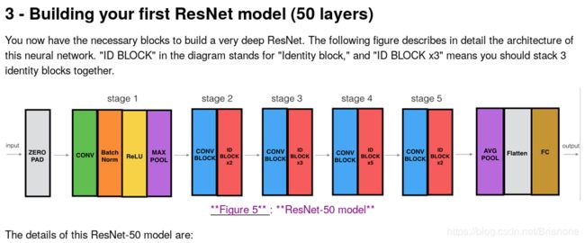
    CONV2D -> BATCHNORM -> RELU -> MAXPOOL -> CONVBLOCK -> IDBLOCK*2 -> CONVBLOCK -> IDBLOCK*3
    -> CONVBLOCK -> IDBLOCK*5 -> CONVBLOCK -> IDBLOCK*2 -> AVGPOOL -> TOPLAYER

    Arguments:
    input_shape -- shape of the images of the dataset
    classes -- integer, number of classes

    Returns:
    model -- a Model() instance in Keras
    """
    
    # Define the input as a tensor with shape input_shape
    X_input = Input(input_shape)

    
    # Zero-Padding
    X = ZeroPadding2D((3, 3))(X_input)
    
    # Stage 1
    X = Conv2D(64, (7, 7), strides = (2, 2), name = 'conv1', kernel_initializer = glorot_uniform(seed=0))(X)
    X = BatchNormalization(axis = 3, name = 'bn_conv1')(X)
    X = Activation('relu')(X)
    X = MaxPooling2D((3, 3), strides=(2, 2))(X)

    # Stage 2
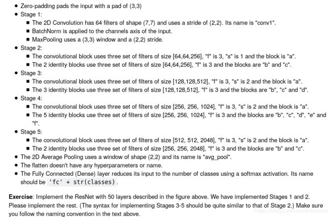
    X = convolutional_block(X, f = 3, filters = [64, 64, 256], stage = 2, block='a', s = 1)
    X = identity_block(X, 3, [64, 64, 256], stage=2, block='b')
    X = identity_block(X, 3, [64, 64, 256], stage=2, block='c')

    ### START CODE HERE ###

    # Stage 3 (≈4 lines)
    # The convolutional block uses three set of filters of size [128,128,512], "f" is 3, "s" is 2 and the block is "a".
    # The 3 identity blocks use three set of filters of size [128,128,512], "f" is 3 and the blocks are "b", "c" and "d".
    X = convolutional_block(X, f=3, filters=[128,128,512], stage=3, block='a', s = 2)
    X = identity_block(X, 3, [128,128,512], stage=3, block='b')
    X = identity_block(X, 3, [128,128,512], stage=3, block='c')
    X = identity_block(X, 3, [128,128,512], stage=3, block='d')
    
    # Stage 4 (≈6 lines)
    # The convolutional block uses three set of filters of size [256, 256, 1024], "f" is 3, "s" is 2 and the block is "a".
    # The 5 identity blocks use three set of filters of size [256, 256, 1024], "f" is 3 and the blocks are "b", "c", "d", "e" and "f".
    X = convolutional_block(X, f=3, filters=[256,256,1024], stage=4, block='a', s = 2) 
    X = identity_block(X, 3, [256,256,1024], stage=4, block='b')
    X = identity_block(X, 3, [256,256,1024], stage=4, block='c')
    X = identity_block(X, 3, [256,256,1024], stage=4, block='d')
    X = identity_block(X, 3, [256,256,1024], stage=4, block='e')
    X = identity_block(X, 3, [256,256,1024], stage=4, block='f')
    

    # Stage 5 (≈3 lines)
    # The convolutional block uses three set of filters of size [512, 512, 2048], "f" is 3, "s" is 2 and the block is "a".
    # The 2 identity blocks use three set of filters of size [256, 256, 2048], "f" is 3 and the blocks are "b" and "c".
    X = convolutional_block(X, f=3, filters=[512,512,2048], stage=5, block='a', s = 2) 
    
    # filters should be [256, 256, 2048], but it fail to be graded. Use [512, 512, 2048] to pass the grading
    X = identity_block(X, 3, [256,256,2048], stage=5, block='b')
    X = identity_block(X, 3, [256,256,2048], stage=5, block='c')

    # AVGPOOL (≈1 line). Use "X = AveragePooling2D(...)(X)"
    # The 2D Average Pooling uses a window of shape (2,2) and its name is "avg_pool".
    X = AveragePooling2D(pool_size=(2,2), name="avg_pool")(X)
    
    ### END CODE HERE ###

    # output layer
    X = Flatten()(X)
    X = Dense(classes, activation='softmax', name='fc' + str(classes), kernel_initializer = glorot_uniform(seed=0))(X)
    
    
    # Create model
    model = Model(inputs = X_input, outputs = X, name='ResNet50')

    return model

model = ResNet50(input_shape = (64, 64, 3), classes = 6)

model.compile(optimizer='adam', loss='categorical_crossentropy', metrics=['accuracy'])

X_train_orig, Y_train_orig, X_test_orig, Y_test_orig, classes = load_dataset()

# Normalize image vectors
X_train = X_train_orig/255.
X_test = X_test_orig/255.

# Convert training and test labels to one hot matrices
Y_train = convert_to_one_hot(Y_train_orig, 6).T
Y_test = convert_to_one_hot(Y_test_orig, 6).T

print ("number of training examples = " + str(X_train.shape[0]))
print ("number of test examples = " + str(X_test.shape[0]))
print ("X_train shape: " + str(X_train.shape))
print ("Y_train shape: " + str(Y_train.shape))
print ("X_test shape: " + str(X_test.shape))
print ("Y_test shape: " + str(Y_test.shape))

number of training examples = 1080
number of test examples = 120
X_train shape: (1080, 64, 64, 3)
Y_train shape: (1080, 6)
X_test shape: (120, 64, 64, 3)
Y_test shape: (120, 6)

model.fit(X_train, Y_train, epochs = 20, batch_size = 32)

Epoch 1/20
1080/1080 [==============================] - 10s 9ms/step - loss: 1.6261 - acc: 0.5204
Epoch 2/20
1080/1080 [==============================] - 2s 2ms/step - loss: 0.5404 - acc: 0.8352
Epoch 3/20
1080/1080 [==============================] - 2s 2ms/step - loss: 0.4718 - acc: 0.8398
Epoch 4/20
1080/1080 [==============================] - 2s 2ms/step - loss: 0.3301 - acc: 0.9213
Epoch 5/20
1080/1080 [==============================] - 3s 2ms/step - loss: 0.2248 - acc: 0.9222
Epoch 6/20
1080/1080 [==============================] - 3s 2ms/step - loss: 0.1626 - acc: 0.9444
Epoch 7/20
1080/1080 [==============================] - 3s 2ms/step - loss: 0.1395 - acc: 0.9556
Epoch 8/20
1080/1080 [==============================] - 2s 2ms/step - loss: 0.1685 - acc: 0.9528
Epoch 9/20
1080/1080 [==============================] - 3s 2ms/step - loss: 0.5878 - acc: 0.8556
Epoch 10/20
1080/1080 [==============================] - 3s 2ms/step - loss: 0.4128 - acc: 0.8806
Epoch 11/20
1080/1080 [==============================] - 3s 2ms/step - loss: 0.2587 - acc: 0.9083
Epoch 12/20
1080/1080 [==============================] - 3s 2ms/step - loss: 0.0995 - acc: 0.9713
Epoch 13/20
1080/1080 [==============================] - 3s 2ms/step - loss: 0.0536 - acc: 0.9806
Epoch 14/20
1080/1080 [==============================] - 3s 2ms/step - loss: 0.0329 - acc: 0.9889
Epoch 15/20
1080/1080 [==============================] - 3s 2ms/step - loss: 0.0213 - acc: 0.9926
Epoch 16/20
1080/1080 [==============================] - 3s 2ms/step - loss: 0.0828 - acc: 0.9741
Epoch 17/20
1080/1080 [==============================] - 3s 2ms/step - loss: 0.0734 - acc: 0.9694
Epoch 18/20
1080/1080 [==============================] - 3s 2ms/step - loss: 0.0318 - acc: 0.9898
Epoch 19/20
1080/1080 [==============================] - 3s 2ms/step - loss: 0.0194 - acc: 0.9963
Epoch 20/20
1080/1080 [==============================] - 3s 2ms/step - loss: 0.0086 - acc: 0.9972

reds = model.evaluate(X_test, Y_test)
print ("Loss = " + str(preds[0]))
print ("Test Accuracy = " + str(preds[1]))

120/120 [==============================] - 1s 6ms/step
Loss = 0.054361330717802046
Test Accuracy = 0.975

model = load_model('ResNet50.h5') 

preds = model.evaluate(X_test, Y_test)
print ("Loss = " + str(preds[0]))
print ("Test Accuracy = " + str(preds[1]))

 

img_path = 'images/my_image.jpg'
img = image.load_img(img_path, target_size=(64, 64))
x = image.img_to_array(img)
x = np.expand_dims(x, axis=0)
x = preprocess_input(x)
print('Input image shape:', x.shape)
my_image = scipy.misc.imread(img_path)
imshow(my_image)
print("class prediction vector [p(0), p(1), p(2), p(3), p(4), p(5)] = ")
print(model.predict(x))

 

You can also print a summary of your model by running the following code.

model.summary()

Finally, run the code below to visualize your ResNet50. You can also download a .png picture of your model by going to "File -> Open...-> model.png".

plot_model(model, to_file='model.png')
SVG(model_to_dot(model).create(prog='dot', format='svg'))