SPM12 核磁数据预处理 傻瓜攻略

写在最前：鉴于我自己脑子傻，请不要迷信这篇文章的方法的正确性，数据分析的方法真的很多，基于数据的差异可能在一些地方的设置或数据处理步骤都会有差异！也希望发现这篇文章哪里有错误或可以改进的大神可以评论指出，蟹蟹~
人生最痛苦的事不是没得选择，而是选择太多而不知道究竟哪个是对的。这份傻瓜攻略写给我自己，因为我真的服了自己的脑子了。咋么能这么傻呢？
希望有人看到这篇文章之后可以不需要再看其它的文章就可以顺利地从头分析到尾。也希望我不要下一次分析的时候又忘了这些经验。
当然，要是想知道更加具体的原理之类的还是要出门左拐。
SPM（Statistical Parametric Mapping，http://www.fil.ion.ucl.ac.uk/spm/）已经拥有挺久的历史了，这个软件出名的原因，在我看来有两个，一个是算得准，一个是比较容易使用。需要写代码使用的东西就容易用户不友好。所以这样就可以逆推出SPM是一款操作简单的软件，适合小白入门。
如果BOLD 功能图像的扫描方式是间隔采样，先做slice timing，后做realignment；如是顺序采样，则先做realignment 后做slice timing（原理可以看看关于slice timing顺序的问题）
现在最新版的spm是spm12，本文也是基于spm12进行的功能像的预处理。由于spm从spm8到spm12的版本Normalise发生了一些变化，所以在操作上也有一些差异。
好啦，废话说了太多，以下正文：

总体的分析逻辑

1. Dicom转Nifti，去掉前10个由于机器因素不稳定的时间点，手动将结构像的图像的original定位到AC（前联合），并且如果结构像的方向旋转地太厉害也需要人工调整一下，使用的是SPM中的Display工具，先set orient再reorient。
2. Temporal preprocessing：Slice Timing时间层校正
3. Spatial preprocessing：
   • Realign头动校正，会生成rp开头的头动参数文件，头动过大标准为2mm和2°。
   • Coregister配准（将结构像与功能像位置对准）
   • Segment分割（将与功能像配准的结构像分割成灰质，白质，脑脊液），在这一步的Deformation fields中选择Forward就会把分割的文件normalise到MNI空间（这一点跟VBM分析中使用DARTEL的Normalise
     to MNI是不同的，VBM中使用的是原始的结构像文件而不是与功能像配准后的结构像文件）。Deformation
     field生成的是y开头的nii文件。
   • Normalise归一化，将头动校正后的功能像文件与归一化到MNI空间，这一步就需要用到上一步的y开头的文件。
   • Normalise归一化，再做一次归一化是为了将bia corrected的结构像（在Segment阶段生成的m开头文件）也归一化到MNI空间，这样你就可以把归一化后的功能像w开头文件superimposed到归一化后的结构像w开头的文件上。
   • Smooth平滑，Smooth是一种空间上的滤波，而之后的去线性趋势和低通滤波是时间上的滤波，其作用如下图（图片来自于北京师范大学认知神经科学与学习国家重点实验室的PPT）：
     
4. 下面两步是SPM的预处理过程中没有的，但是一般也需要做，我之后应该会用DPARSF或者REST来做这两步吧，现在这里写出来，避免有人觉得只做到Smooth就结束了

• Detrend去线性趋势，也就是高通滤波（让高频的信号留下来，而把低频的信号去掉就叫做高通滤波，反之就叫做低通滤波），在SPM的1-st level分析中包括了这一步，所以如果处理的是任务态的功能像数据就可以只使用SPM了。
• Filter低频滤波（0.01~0.08Hz）和去除协变量，这一步多用在静息态的数据处理中。
  与时间上的滤波相关的问题：Temporal Filtering FAQ

步骤1： 安装好Matlab

（要用SPM12这个版本的话要是Matlab2012以后的版本，我之前装的2016b按道理是可以的，但是后来legend函数更新失败，导致realignment部分报错，在运行batch的时候会出现问题，所以安装的时候最好是能装新的就装新的版本。）
ps：注意matlab的安装路径，以及之后工作的路径都不要有中文，虽然matlab支持中文，但是很多时候还是会出现这样那样的问题。

步骤2： 下载SPM12

，然后把它解压到Matlab的安装地址下的toolbox文件夹中，最后的样子就是下图这样：

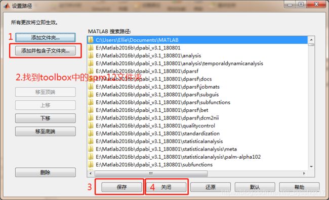
步骤3： 设置SPM的路径

打开matlab，在设置路径（下面第一幅图）中，选择“添加并包含子文件夹”，找到toolbox中的spm12文件夹，然后点击保存，最后关闭（看下面第二幅图）。现在你就可以开始使用SPM12了。

步骤4： 整理核磁数据文件

把你的核磁数据都转成nii的格式，这一步可以使用SPM中的Dicom Import，也可以选用其它的方法。总之，最后你需要把文件的格式整理成下图的形式：
然后，强烈建议整个data文件夹先备份一份。接着删除每个session的前10个时间点（也就是前十个nii文件，这里不一定是10个，按照需要可以删掉8~12个）。
手动将结构像的图像的original定位到AC（前联合），并且如果结构像的方向旋转地太厉害也需要人工调整一下，使用的是SPM中的Display工具，先set orient再reorient。

步骤5： 把Matlab的工作路径改成data文件夹的地址

（如图），在Matlab的命令行窗口输入：spm fmri 然后回车，这样就会打开SPM12分析核磁数据的窗口了。如果你只输入spm，然后回车的话就会出现几个选项，其中有fmri，点击那个按钮也可以打开分析核磁数据的窗口。

步骤6： 开始分析

点击Menu窗口中的Batch，打开了一个Batch editor界面，然后在其中的SPM中分别选择 ① SPM-Temporal-Slice Timing（下面第二张图，其它选择方法类似） ② SPM-Spatial-Realign-Realign：Estimate & Reslice ③ SPM-Spatial-Coregister-Coregister：Estimate ④ SPM-Spatial-Segment ⑤ SPM-Spatial-Normalise-Normalise：Write ⑥ SPM-Spatial-Normalise-Normalise：Write ⑦ SPM-Spatial-Smooth。最后的界面就如下面第三张图片所示。
注意：Normalise：Write要选两次，然后这些modules的顺序不要搞乱了！

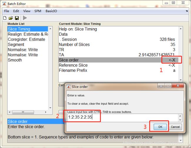
步骤7： Slice Timing

选中Slice Timing这个module，然后设置参数如下：

• 双击Data建立新的session，然后双击session后的<-X打开一个界面，添加单个session文件夹中的所有原始功能像.nii文件（如图一）。
• Number of Slices是nii文件的扫描时的层数，我这里是35层。
• TR为Time of Repetition，可以通过matlab中的dicominfo(‘XXX’)命令来查看，其中XXX为dicom文件的全写，最好包括文件的绝对地址，注意要加单引号。我这里的TR为3（单位是秒）。
• TA=TR-TR/(Number of Slices)，所以在这里是3-3/35（如图二）。
• Slice order为[1:2:number_of_slices 2:2:number_of_slices]，所以这里填入1:2:35 2:2:35（如图三）
• Reference Slice设置为中间时间扫描的那一层，我们注意到在Slice order部分最后生产的矩阵为[1 3 5 7 9 11 13 15 17 19 21 23 25 27 29 31 33 35 2 4 6 8 10 12 14 16 18 20 22 24 26 28 30 32 34]，所以中间时刻扫描的层是第35层，所以Reference Slice设为35。
  最后所有Slice Timing的参数都设置好了，最终如下面第四张图所示

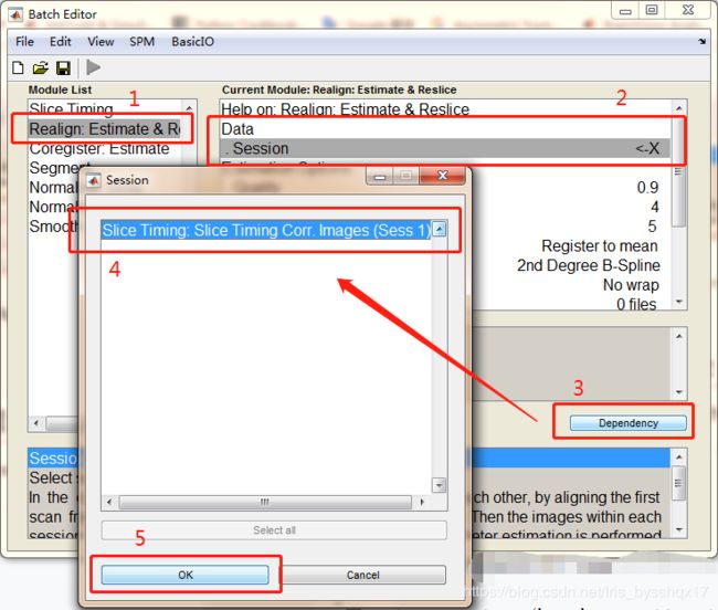
步骤8： Realignment

选中Realign：Estimate & Reslice这个module，然后设置参数如下：

• 双击Data建立新的Session，单击Session后面的<-X，选择Dependency，选择新的页面中上一步Slice Timing（时间层校正）后的文件，点击OK。
• 其它部分都按照默认就好了，注意，Resliced images中默认选择的是All Images+Mean Image，不要去改这个！
  最后所有Realign：Estimate&Reslices的参数都设置好了，最终如下面第二张图所示
  
  

步骤9： Coregister

选中Coregister：Estimate这个module，然后设置参数如下：

• Reference Image选择Dependency中的Realign：Estimate & Reslice: Mean Image，也就是上一步的Realign过后生成的mean开头的文件，如下面第一张图。
• Source Image选择原始的结构像文件，如下面第二张图。双击Source Image后面的<-X，找到当前的被试所对应的的structure文件夹中的结构像的nii文件。
  最后所有Coregister：Estimate的参数都设置好了，最终如下面第三张图所示
  
  
  

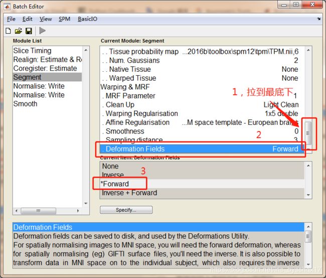
步骤10： Segment

选中Segment这个module，然后设置参数如下：

• Volumes选择Dependency中的Coregister: Estimate: Coregistered Images，也就是上一步Coregister完后生成的文件。
• 将Save Bias Corrected部分由Save Nothing改为Save bias corrected，如下面第二幅图。
• 将Deformation Fields部分由Nothing改为Forward，如下面第三幅图所示。
  到这里所有Segment的参数都设置好了
  
  
  

步骤11： Normalise (1)

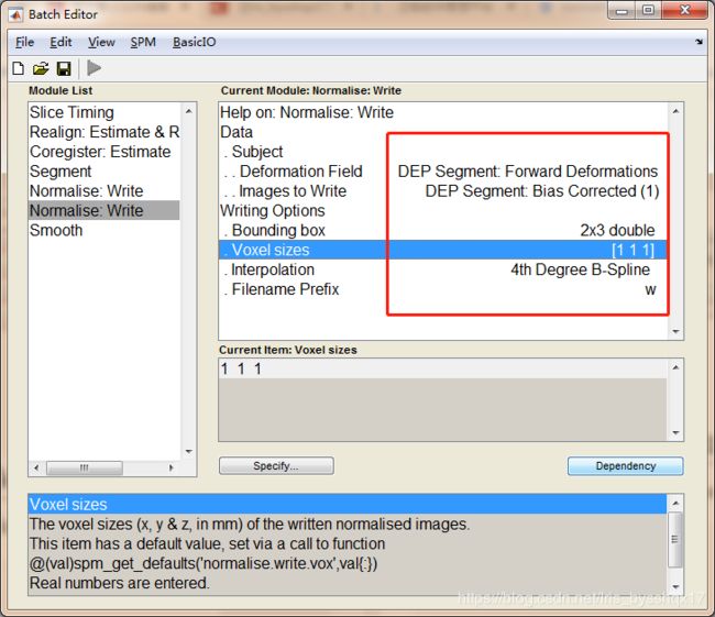
选中第一个Normalise: Write这个module，然后设置参数如下：

• Deformation Field选择Dependency中的Segment: Forward Deformations，也就是上一步在Deformation中选择了Forward之后生成的文件，如下面第一张图。
• Images to write选择Dependency中的Realign: Estimate & Reslice: Realigned Images (Sess 1)，也就是Realign（头动矫正）过的所有功能像的开头为r的.nii文件，如下面第二张图。
• 将Voxel sizes由默认的[2 2 2]改为[3 3 3]
  最后所有第一个Normalise: Write的参数都设置好了，最终如下面第三张图所示
  
  
  

步骤12： Normalise (2)

选中第二个Normalise: Write这个module，然后设置参数如下：

• Deformation Field还是选择Dependency中的Segment: Forward Deformations，如下面第一张图。
• Images to Write选择Dependency中的Segment: Bias Corrected (1)，也就是bias-corrected完的结构像的开头为m的文件，如下面第二张图。
• 将Voxel sizes由默认的[2 2 2]改为[1 1 1]，这个数字是结构像原本的分辨率。
  最后所有第二个Normalise: Write的参数都设置好了，最终如下面第三张图所示
  
  
  

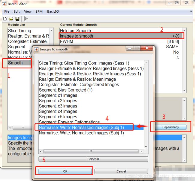
步骤13： Smooth

选中Smooth这个module，然后设置参数如下：

• Images to smooth选择Dependency中的Normalise: Write: Normalised Images (Subj 1)中的第一个，如下面第一张图。
• FWHM改成[6 6 6]，为Normalise中选择的Voxel sizes的[3 3 3]的两倍。
  最后所有Smooth的参数都设置好了，最终如下面第二张图所示
  
  

步骤14： 运行Batch

保存这个batch文件为preprocessing.mat，然后单击绿色的箭头开始run这个预处理，接下来只需要等着处理完成了~
如果你只需要分析一个数据的话，到这一步就可以了，但是一般来说，核磁数据分析都是一个批次从十几个到几百个不等。每一次都要重新走一遍这个流程，尽管只需要改一下原始数据或者几个参数。但是一来这样操作很可能由于手误而出现问题，而且后期的检查很难察觉，二来也比较麻烦。由此看来，对数据的批量处理是很有必要的。如果你需要批量处理，就往下看吧。

接下来会写怎么写一个m文件，可以一次性把所有被试的数据都做好预处理，而不需要每一个都做一遍上面的步骤。

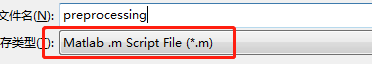
步骤15： 建立m文件

把刚刚的batch另存为matlab .m Script格式，然后打开这个preprocessing.m文件。

打开的文件是下面这样的：

步骤16： 修改m文件

先看一下下面这个维基百科上面对于Batch的建议：

基于一个session的预处理的m文件如下：

%-----------------------------------------------------------------------
% Job saved on 02-Sep-2019 18:21:16 by cfg_util (rev $Rev: 6942 $)
% spm SPM - SPM12 (7219)
% cfg_basicio BasicIO - Unknown
%-----------------------------------------------------------------------
%%
% 这个m文件用来运行spm的matlabbatch
% 该文件中的文件位置是基于linux系统的，如果是windows系统需要修改/为\
clear
% spm_path = '~/spm12';      %设置spm12的位置（这里填的是安装=spm12的绝对位置）
% addpath(spm_path);
spm('defaults', 'fmri');
spm_jobman('initcfg');

%%
subjectsdir = {'~/data'};                      % 这里是data文件夹的绝对位置
subjects = {'sbj01','sbj02','sbj03'};          % 单个或多个被试的文件夹
funcdir  =  fullfile('Session1');              % 第一个Session的文件夹（由于preprocessing.mat中只添加了一个Session，所以这里也只使用一个Session。）
% funcdir2  =  fullfile('Session2');             % 第二个Session的文件夹
anatdir =  fullfile('Structure');              % 结构像的文件夹

%%
% 设置基本的参数，在这里设置方便后期修改
slice_number = 35;
TR = 3;
TA = TR-TR/slice_number;
slice_order = [1:2:slice_number 2:2:slice_number];
refslice1 = 35;
voxel_size= [3.75 3.75 4];
smoothing_kernel = [6 6 6];

%%
%每一个被试都建立一个工作流程

nsubj = length(subjects);   % 被试的数量
jobs = cell(nsubj,1);       % job的数量，每个被试一个job
nrun=1;  % session的数量
ntimepoint=190;  %删除了前面的10个时间点后剩余的时间点
%%
for csubj = 1:nsubj
    subjdir = {spm_select('CPath', subjects{csubj}, subjectsdir)};
    % 结构像文件夹
    adir =  spm_select('CPath', anatdir, subjdir);   %选择当前被试（csubj）的结构像文件夹
    anatfile = strcat(spm_select('FPList', adir, '/*.nii'),',1');   %在这个文件夹中.nii结尾的文件，即结构像文件
    %如果没有结构像文件就报错
    if isequal(anatfile,  '')
        warning(sprintf('No anat file found for %s', ...
            subjects{csubj}))
        return
    end
    % Session1文件夹
    fdir =  {spm_select('CPath', funcdir, subjdir)};    %选择当前被试（csubj）的Session1文件夹
    ffiles = spm_select('List', fdir, '/*.nii');   %选择这个文件夹中所有.nii结尾的文件，即Session1的所有原始功能像文件
    %如果没有功能像文件就报错
    nimage = size(ffiles,1);
    if nimage == 0
        warning(sprintf('No functional file found for %s', subjects{csubj}))
        return
    end
    funcfiles = cell(1, nrun);
    sessionfiles = cell(nrun,ntimepoint);
    cffiles = cellstr(ffiles);
    for i = 1:nrun
        for j = 1:ntimepoint
            sessionfiles{i,j}=strcat(fdir{1},'/',cffiles{j},',1');   % 在这里在每一个功能像文件的绝对路径后面添加,1
        end
        funcfiles{1,i} = {sessionfiles{i,:}}';    % 如果有多个Sessions，funcfiles中就会有多个sessionfiles
    end
    clear matlabbatch
    
    % preprocessing job
    display 'Creating preprocessing job'  %在matlab的命令行窗口显示Creating preprocessing job
    
    % Slice Timing
    matlabbatch{1}.spm.temporal.st.scans = {funcfiles{:}};   %把这里的文件换成上面设置的funcfiles
    matlabbatch{1}.spm.temporal.st.nslices = slice_number;   %把这里原先的数字35修改为slice_number这个变量，以下操作类似
    matlabbatch{1}.spm.temporal.st.tr = TR;              %修改TA
    matlabbatch{1}.spm.temporal.st.ta = TA;              %修改TR
    matlabbatch{1}.spm.temporal.st.so = slice_order;     %修改slice_order
    matlabbatch{1}.spm.temporal.st.refslice = refslice1;     %修改refslice1
    matlabbatch{1}.spm.temporal.st.prefix = 'a';
    
    % Realign
    matlabbatch{2}.spm.spatial.realign.estwrite.data{1}(1) = cfg_dep('Slice Timing: Slice Timing Corr. Images (Sess 1)', substruct('.','val', '{}',{1}, '.','val', '{}',{1}, '.','val', '{}',{1}), substruct('()',{1}, '.','files'));
    matlabbatch{2}.spm.spatial.realign.estwrite.eoptions.quality = 0.9;
    matlabbatch{2}.spm.spatial.realign.estwrite.eoptions.sep = 4;
    matlabbatch{2}.spm.spatial.realign.estwrite.eoptions.fwhm = 5;
    matlabbatch{2}.spm.spatial.realign.estwrite.eoptions.rtm = 1;
    matlabbatch{2}.spm.spatial.realign.estwrite.eoptions.interp = 2;
    matlabbatch{2}.spm.spatial.realign.estwrite.eoptions.wrap = [0 0 0];
    matlabbatch{2}.spm.spatial.realign.estwrite.eoptions.weight = '';
    matlabbatch{2}.spm.spatial.realign.estwrite.roptions.which = [2 1];
    matlabbatch{2}.spm.spatial.realign.estwrite.roptions.interp = 4;
    matlabbatch{2}.spm.spatial.realign.estwrite.roptions.wrap = [0 0 0];
    matlabbatch{2}.spm.spatial.realign.estwrite.roptions.mask = 1;
    matlabbatch{2}.spm.spatial.realign.estwrite.roptions.prefix = 'r';
    
    % Coregister
    matlabbatch{3}.spm.spatial.coreg.estimate.ref(1) = cfg_dep('Realign: Estimate & Reslice: Mean Image', substruct('.','val', '{}',{2}, '.','val', '{}',{1}, '.','val', '{}',{1}, '.','val', '{}',{1}), substruct('.','rmean'));
    matlabbatch{3}.spm.spatial.coreg.estimate.source = {anatfile}; %这里是结构像文件
    matlabbatch{3}.spm.spatial.coreg.estimate.other = {''};
    matlabbatch{3}.spm.spatial.coreg.estimate.eoptions.cost_fun = 'nmi';
    matlabbatch{3}.spm.spatial.coreg.estimate.eoptions.sep = [4 2];
    matlabbatch{3}.spm.spatial.coreg.estimate.eoptions.tol = [0.02 0.02 0.02 0.001 0.001 0.001 0.01 0.01 0.01 0.001 0.001 0.001];
    matlabbatch{3}.spm.spatial.coreg.estimate.eoptions.fwhm = [7 7];
    matlabbatch{4}.spm.spatial.preproc.channel.vols(1) = cfg_dep('Coregister: Estimate: Coregistered Images', substruct('.','val', '{}',{3}, '.','val', '{}',{1}, '.','val', '{}',{1}, '.','val', '{}',{1}), substruct('.','cfiles'));
    
    % Segment
    matlabbatch{4}.spm.spatial.preproc.channel.biasreg = 0.001;
    matlabbatch{4}.spm.spatial.preproc.channel.biasfwhm = 60;
    matlabbatch{4}.spm.spatial.preproc.channel.write = [0 1];
    matlabbatch{4}.spm.spatial.preproc.tissue(1).tpm = {'~/Matlab2016b/toolbox/spm12/tpm/TPM.nii,1'}; % 这里是spm12默认的TPM.nii文件的位置，以下类似
    matlabbatch{4}.spm.spatial.preproc.tissue(1).ngaus = 1;
    matlabbatch{4}.spm.spatial.preproc.tissue(1).native = [1 0];
    matlabbatch{4}.spm.spatial.preproc.tissue(1).warped = [0 0];
    matlabbatch{4}.spm.spatial.preproc.tissue(2).tpm = {'~/Matlab2016b/toolbox/spm12/tpm/TPM.nii,2'};
    matlabbatch{4}.spm.spatial.preproc.tissue(2).ngaus = 1;
    matlabbatch{4}.spm.spatial.preproc.tissue(2).native = [1 0];
    matlabbatch{4}.spm.spatial.preproc.tissue(2).warped = [0 0];
    matlabbatch{4}.spm.spatial.preproc.tissue(3).tpm = {'~/Matlab2016b/toolbox/spm12/tpm/TPM.nii,3'};
    matlabbatch{4}.spm.spatial.preproc.tissue(3).ngaus = 2;
    matlabbatch{4}.spm.spatial.preproc.tissue(3).native = [1 0];
    matlabbatch{4}.spm.spatial.preproc.tissue(3).warped = [0 0];
    matlabbatch{4}.spm.spatial.preproc.tissue(4).tpm = {'~/Matlab2016b/toolbox/spm12/tpm/TPM.nii,4'};
    matlabbatch{4}.spm.spatial.preproc.tissue(4).ngaus = 3;
    matlabbatch{4}.spm.spatial.preproc.tissue(4).native = [1 0];
    matlabbatch{4}.spm.spatial.preproc.tissue(4).warped = [0 0];
    matlabbatch{4}.spm.spatial.preproc.tissue(5).tpm = {'~/Matlab2016b/toolbox/spm12/tpm/TPM.nii,5'};
    matlabbatch{4}.spm.spatial.preproc.tissue(5).ngaus = 4;
    matlabbatch{4}.spm.spatial.preproc.tissue(5).native = [1 0];
    matlabbatch{4}.spm.spatial.preproc.tissue(5).warped = [0 0];
    matlabbatch{4}.spm.spatial.preproc.tissue(6).tpm = {'~/Matlab2016b/toolbox/spm12/tpm/TPM.nii,6'};
    matlabbatch{4}.spm.spatial.preproc.tissue(6).ngaus = 2;
    matlabbatch{4}.spm.spatial.preproc.tissue(6).native = [0 0];
    matlabbatch{4}.spm.spatial.preproc.tissue(6).warped = [0 0];
    matlabbatch{4}.spm.spatial.preproc.warp.mrf = 1;
    matlabbatch{4}.spm.spatial.preproc.warp.cleanup = 1;
    matlabbatch{4}.spm.spatial.preproc.warp.reg = [0 0.001 0.5 0.05 0.2];
    matlabbatch{4}.spm.spatial.preproc.warp.affreg = 'mni';
    matlabbatch{4}.spm.spatial.preproc.warp.fwhm = 0;
    matlabbatch{4}.spm.spatial.preproc.warp.samp = 3;
    matlabbatch{4}.spm.spatial.preproc.warp.write = [0 1];
    
    % Normalise 1
    matlabbatch{5}.spm.spatial.normalise.write.subj.def(1) = cfg_dep('Segment: Forward Deformations', substruct('.','val', '{}',{4}, '.','val', '{}',{1}, '.','val', '{}',{1}), substruct('.','fordef', '()',{':'}));
    matlabbatch{5}.spm.spatial.normalise.write.subj.resample(1) = cfg_dep('Realign: Estimate & Reslice: Realigned Images (Sess 1)', substruct('.','val', '{}',{2}, '.','val', '{}',{1}, '.','val', '{}',{1}, '.','val', '{}',{1}), substruct('.','sess', '()',{1}, '.','cfiles'));
    matlabbatch{5}.spm.spatial.normalise.write.woptions.bb = [-78 -112 -70
        78 76 85];
    matlabbatch{5}.spm.spatial.normalise.write.woptions.vox = [3 3 3];
    matlabbatch{5}.spm.spatial.normalise.write.woptions.interp = 4;
    matlabbatch{5}.spm.spatial.normalise.write.woptions.prefix = 'w';
    
    % Normalise 2
    matlabbatch{6}.spm.spatial.normalise.write.subj.def(1) = cfg_dep('Segment: Forward Deformations', substruct('.','val', '{}',{4}, '.','val', '{}',{1}, '.','val', '{}',{1}), substruct('.','fordef', '()',{':'}));
    matlabbatch{6}.spm.spatial.normalise.write.subj.resample(1) = cfg_dep('Segment: Bias Corrected (1)', substruct('.','val', '{}',{4}, '.','val', '{}',{1}, '.','val', '{}',{1}), substruct('.','channel', '()',{1}, '.','biascorr', '()',{':'}));
    matlabbatch{6}.spm.spatial.normalise.write.woptions.bb = [-78 -112 -70
        78 76 85];
    matlabbatch{6}.spm.spatial.normalise.write.woptions.vox = [1 1 1];
    matlabbatch{6}.spm.spatial.normalise.write.woptions.interp = 4;
    matlabbatch{6}.spm.spatial.normalise.write.woptions.prefix = 'w';
    
    % Smooth
    matlabbatch{7}.spm.spatial.smooth.data(1) = cfg_dep('Normalise: Write: Normalised Images (Subj 1)', substruct('.','val', '{}',{5}, '.','val', '{}',{1}, '.','val', '{}',{1}, '.','val', '{}',{1}), substruct('()',{1}, '.','files'));
    matlabbatch{7}.spm.spatial.smooth.fwhm = smoothing_kernel;   % 修改smoothing_kernel
    matlabbatch{7}.spm.spatial.smooth.dtype = 0;
    matlabbatch{7}.spm.spatial.smooth.im = 0;
    matlabbatch{7}.spm.spatial.smooth.prefix = 's';
    
    % 保存matlabbatch
    matfile = sprintf('preprocess_%s.mat', subjects{csubj});
    save(matfile,'matlabbatch');
    jobs{csubj} = matfile;  %jobs这个变量中存储了所有被试的matlabbatch
end

%%
% 执行预处理的工作
for csubj = 1:nsubj
    display 'Start preprocessing job'   %在matlab的命令行窗口显示Start preprocessing job
    spm_jobman('run', jobs{csubj});
end

要非常注意的地方是功能像文件那个变量funcfiles的格式，以及其中的sessionfiles还有cffiles两个变量的格式！问题常常出现在这里。

最后推荐一个我觉得相对较好的教程（是英文的）：
WIKIBooks上面的SPM教程
然后就是SPM12的手册，在SPM的安装包中自带的，位置是文件夹~/spm12/man/manual.pdf

补充

Realign 后生成的rp头动参数文件，前三列是平动，后三列是转动。
要找出最大的头动参数可以使用下面的代码：

%%这个代码运行在matlab中，其中的rp_name.txt是指生成的rp文件
b=load(‘rp_name.txt’);       %调入头动文件
c=max(abs(b));             %取头动的最大值,即六列数每列中最大的数，共六个数
c(4:6)=c(4:6)*180/pi;        %把后三个数(转动数据)的单位由弧度换成度

要找出大于某个标准（比如2mm，2°），可以将rp文件放入excel中，先将后三列使用X*180/π转成角度，然后使用IF(X>2,1,0)来找出超过标准的值。