李宏毅机器学习Lecture 1：回归 - 案例研究

ML Lecture 1: Regression - Case Study

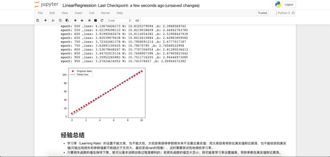
本笔记有配套的Jupyter Notebook演练，包含tensorflow基础api实现的单变量线性回归与多元线性回归，以及对梯度下降训练过程的改进讲解，同时包括高级lib如sklearn与keras的线性回归实现。欢迎在读完笔记后去实际演练一下哟~

如果觉得本系列文章对您有帮助的话，麻烦不吝在对应的github项目上点个star吧！非常感谢！您的支持就是我继续创作的动力哟！

• Application Examples of Regression

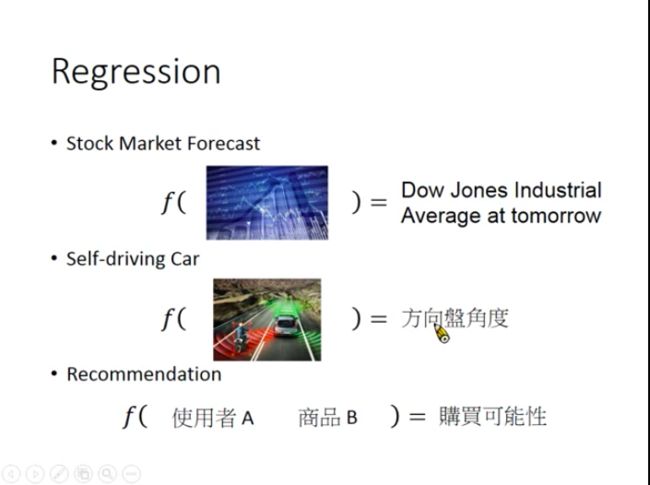
In Reality: stock market forecast, self-driving car and recommendation.

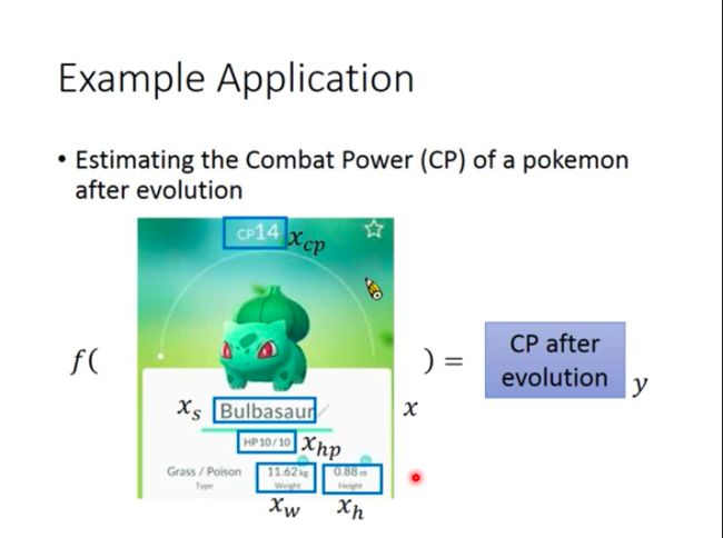
In Pokemon: estimating the Combat Power (CP) of a Pokemon after evolution.

Steps to do Regression

Step 1: Model

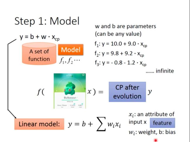
Define a model (a set of function) that maps x to y, different parameters make different functions, and we need training data to tell us the right parameter values.

• Linear Model

As long as relationship between y and x can be written as:
$$y=b+\Sigma w_i{x}_i$$
Here, $x_i$ is an attribute of input x (also known as feature). $w_i$ called weight and $b$ called bias. Then, we call this kind of model linear model.

Step 2: Goodness of Function

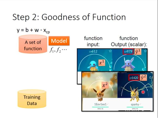
In task of predicting Pokemon CP, we need to collect lots of data consisting of CP before and after Pokemon evolve.

$x^1$ stands for CP before evolution/original CP (‘1’ as superscript stands for a single example marked as 1). ${\hat{y}}^1$ stands for CP after evolution (hat “^” means this is a real value for the input).

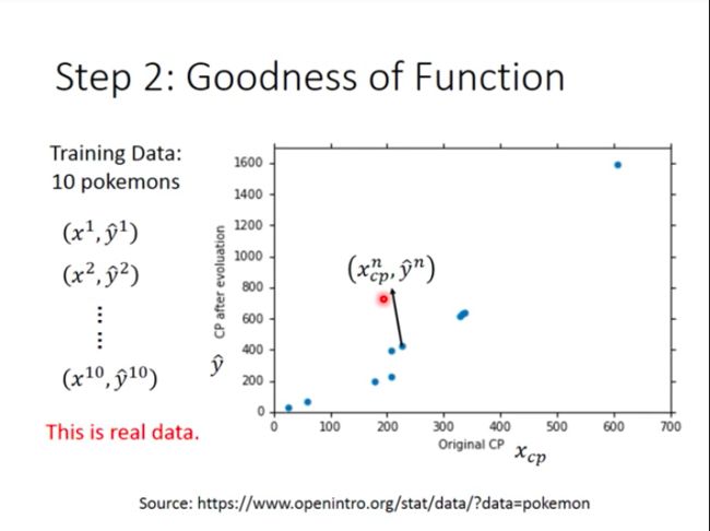
Assume we have 10 training examples:

Every blue point in the coordinate represents a example.

Loss Function L

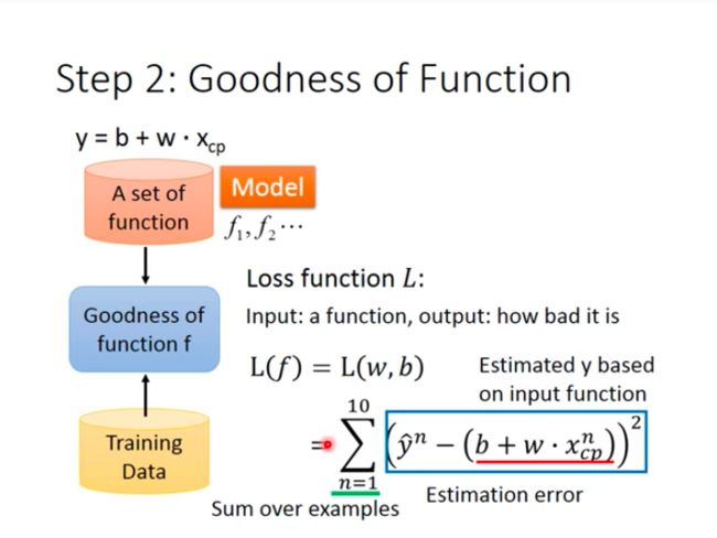
Loss funtion is a “function of function”. Its input is a function while its output is how bad the given function is.

$$L(f)=L(w,b)={\Sigma }_{n=1}^{10}({\hat{y}}^n-(b+w\ast x_{cp}^n){)}^2$$

While function f is defined by paramater b and w, so loss function is actually measuring how bad a set of parameter(w&b) is. And intuitively, the loss function in the slide is summing the difference between estimated y and real y($\hat{y}$) over all 10 examples.

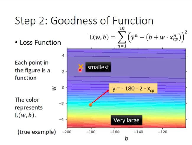
• What does loss function look like?

Every point in the coordinate stands for a function/a set of parameter, and the color in the background stands for value of loss function (from purple to red, the value of loss function rises). As we can see from the coordinate, loss function with smallest value locates at purple region, and that point is the best function that we should pick!

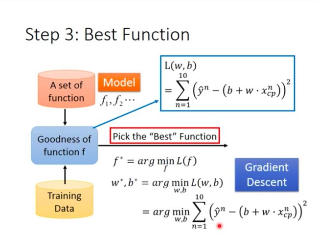
Step 3: Best Function

This step is to pick the “Best” function $f^{\ast }$ that can minimize loss function.

$$f^{\ast }=arg\underset{f}{\min }L(f)$$
$$w^{\ast },b^{\ast }=arg\underset{w,b}{\min }L(w,b)=arg\underset{w,b}{\min }{\Sigma }_{n=1}^{10}({\hat{y}}^n-(b+w\ast s_{cp}^n){)}^2$$

• How to solve above equation so that we can pick the best function?

A: Gradient Descent!

Gradient Descent

As is stated above, we need to find $w^{\ast }$ and $b^{\ast }$ that can minimize loss function, and a obvious way to do this is to exhaust all possible value for w and b, and then calculate loss function’s value. But since it’s obviously not practical since there are countless possible values for w and b. So we turn to gradient descent (GD).

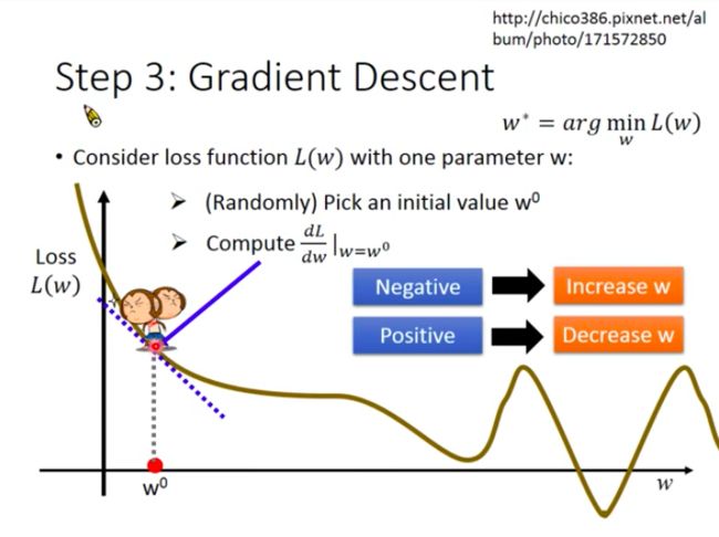
• How do GD work?

For only one parameter:

• Randomly choose a point $w_0$ for w;
• compute $\frac{dL}{dw}{|}_w=w^0$ (tangent slope for the corresponding point on loss function);
• choose the direction that will make value of loss function to decrease and “move a bit”.

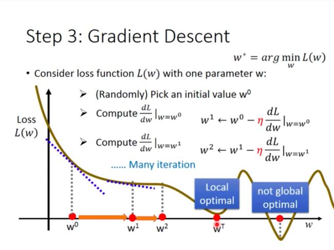
How to decide the moving distance?

• derivative: $\frac{dL}{dW}{|}_w=w^0$
• learning rate $\eta$: a constant value

Then repeat above steps, until the loss function get to a local minimum, but it may not be global minimum:

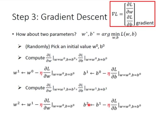
For two parameters:

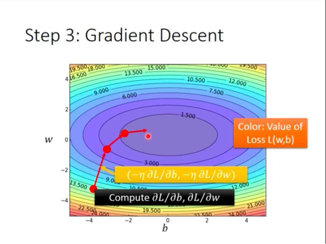
Similarly, compute partial differential for each parameter, and then update two parameter at the same time, then repeat above steps:

Attention: ‘gradient’ here refers to vector stacked by partial differential of different parameters in the function.

Then, Let’s visualize what GD is actually doing where there are two parameters:

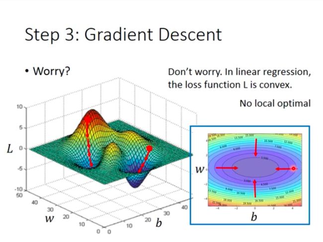
• Worry for GD?

**Different start points may lead you to different results…(Left Picture)**But we don’t have to worry that in linear regression, cause usually there would be only one local minimum, also the global minimum, to reach.

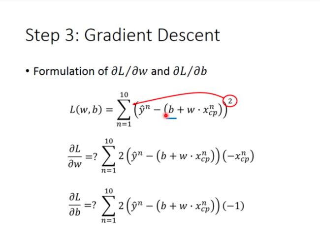
• Formulation of $\partial L/\partial w$ and $\partial L/\partial b$

As long as you have studied calculus before, it’s easy to understand how the formulation comes out:

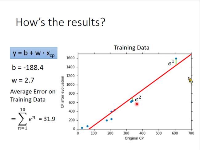
• How’s the results (for Pokemon CP prediction)

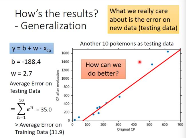
We would get a optimal value for parameter $w$ and $b$, and then we plot the function curve on the coordinate (the red line):

Obviously, the red line can’t perfectly predict Pokemon’s CP, and if you wonder how bad/inaccurate the function is on this task, we can add all error up. Error is the difference between the true CP and estimated CP.

But, this is not what we should pay much attention on, because what we really want the model to do is to predict on Pokemon that it has never seen before (Pokemon data not appeared in training). So, we care more about model’s performance on new data (Testing Data).

• What if we want our model to be perform better?

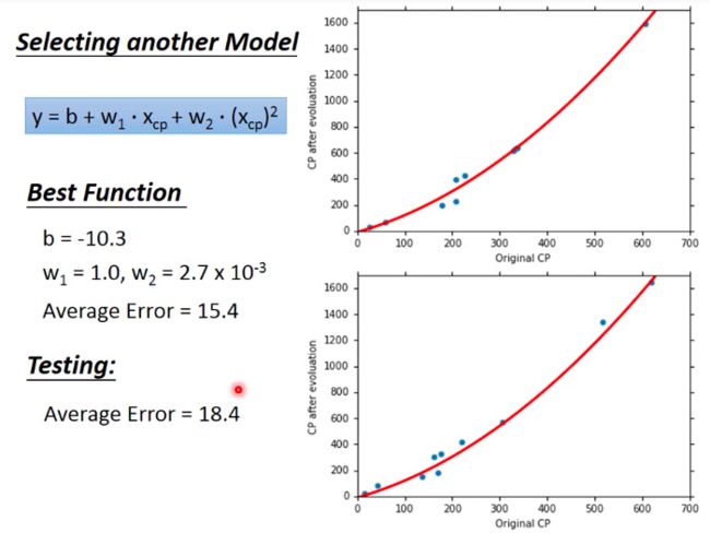
A: Selecting another model!

For example, we could incorporate a new parameter $x_{cp}^2$, then we use the same way mentioned before to obtain optimal values for parameter $b$ and $w$. Still then we plot the function curve together with training data and testing data respectively:

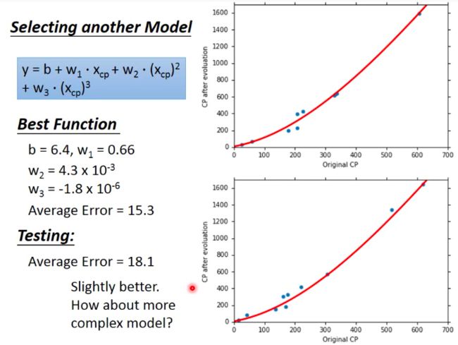
• To make the model more powerful ??

Add $x_{cp}^3$.

Not much difference from last model.

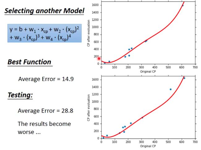
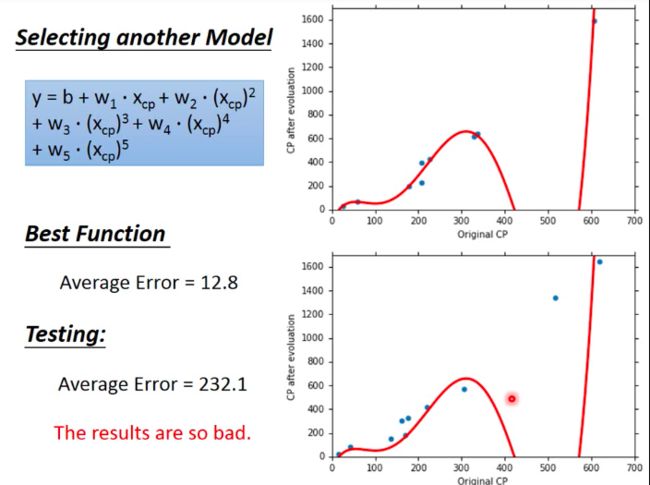
• More powerful? Or Worse?

The performance of models on training data is better then previous one, while the performance on testing data is worse then the previous one!

• Worse!

Model Selection

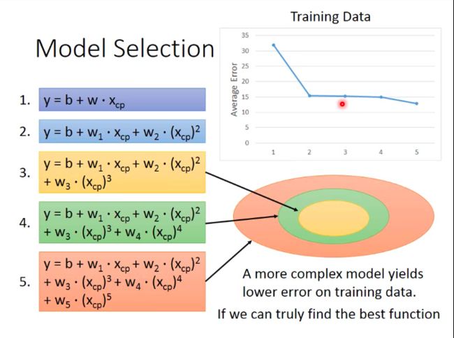
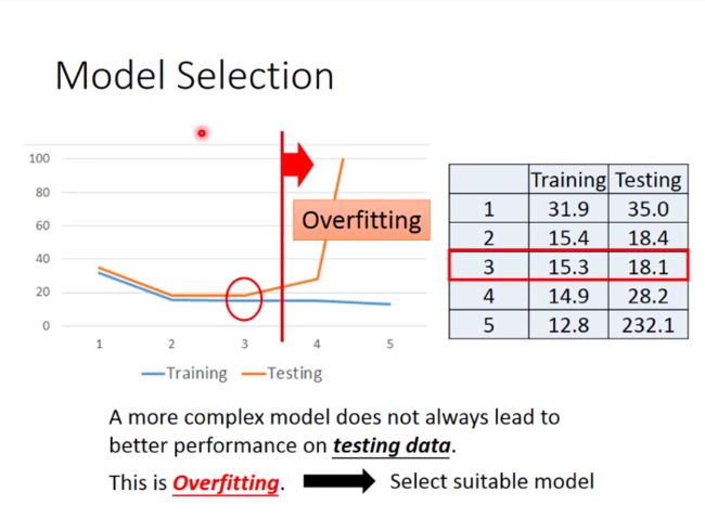
Sort exploration results we’ve got above, We can see from the picture that average error on training data would decrease with the complexity of model. We can intuitively attribute this trend to wider range to choose functions from for complicated model.

But on testing data, we find that more complicated models would perform worse. And this phenomenon (model performing well on training data while bad on testing data) Overfitting.

Prof. Lee offers an example for understanding this intuitively: you learn well about all driving skills to pass the driver 's license testing in particular training environment, but when you get on road without familiar references around, you may encounter various unexpected situations that you’ve never seen before in training.

Therefore, we need to select suitable model!

Collect more data

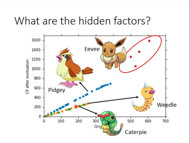
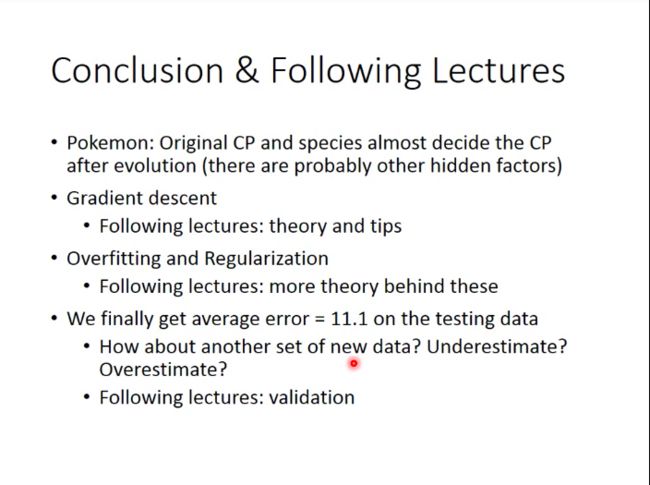
After we collect much more data of Pokemon and plot them on the coordinate, we find that there are some hidden factors that we didn’t take into consideration in our models! In other words, only considering CP before evolution is not enough for predicting CP after evolution!

This also means, we will have to redesign our model to try catching more factors into the model.

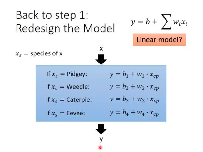
Back to Step 1: Redesign the Model

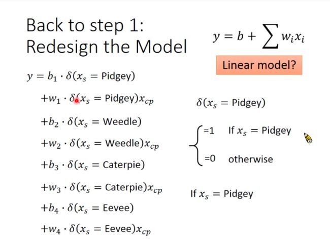
For different specie of Pokemon, we now use different function to fit them:

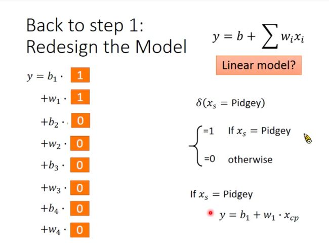
And assemble functions for different Pokemon species:

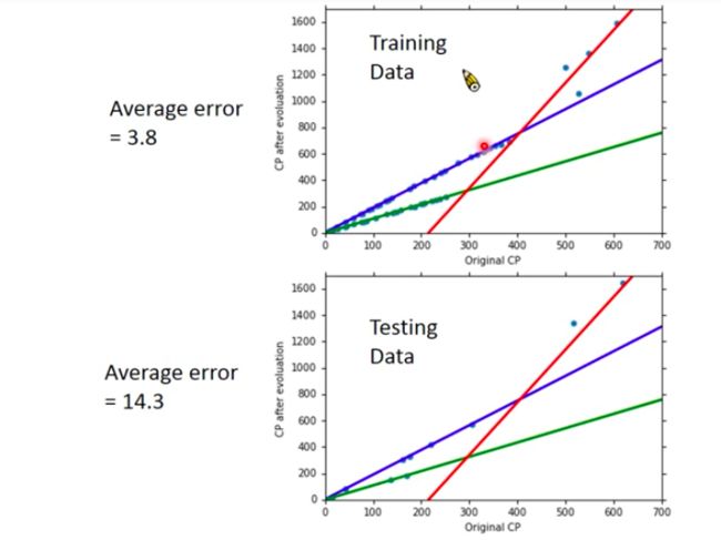
• Results?

Good!

But be careful! There are still some little errors between prediction CP and true CP, which means there are still factors that we haven’t considered. (We could also explain it in this way: Pokemon game may add some random number to value calculated by formulation of CP)

There may also be some other hidden factors: weight, height, HP of Pokemon and so on.

So let’s try improving our model again!

Back to Step 1: Redesign the Model Again

The result is bad on testing data…?

Back to step 2: Regularization

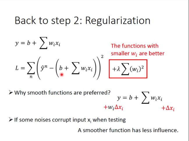
We try adding a new term to our loss function: regularization term. It consists of sum of squares of every $w_i$. This means, if loss function wants to derive a smaller value, $w_i$ needs to be smaller.

From the view of function curve’s shape, smaller $w_i$ means smoother function (same changes in value of $x_i$ would cause less changes in value of $y_i$). So why would we expect smoother functions would perform better? Because there may be noises corrupting input $x_i$ when testing, and a smoother function would has less influence.

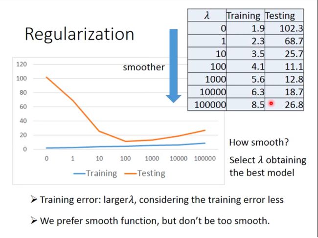
• Results after regularization

We can see from the table, bigger $\lambda$ comes with bigger training error, because bigger $\lambda$ means we pay more attention on smaller parameter values instead of smaller average error. While testing error increases first with $\lambda$ and then decreases, this means our function couldn’t be too smooth either.

So we need to select $\lambda$, i.e. how smooth the function is.

• Why don’t we consider bias term in regularization?

If you try ignoring bias term in experiment, you will get better model performance. The reason is that: we need regularization term to help us obtain smoother function, however, bias term doesn’t relate with the smooth degree of function at all, so we don’t have to incorporate it into regularization.

Concludsion & Following Lectures