语义分割之PointRend论文与源码解读
参考:https://zhuanlan.zhihu.com/p/98508347?utm_source=qq
存在问题:
一般的语义分割网络,在得到一定分辨率的mask之后,都会直接插值回原像素尺寸,这会导致回插的物体边缘像素十分不准确。
以MaskRCNN举例,由于计算量和显存的原因,对于每一个ROIAlign之后的proposal我们一般只会upsample到28*28的分辨率的mask,这对于绝大多数物体显然是不够的,然后插值回原图片大小,导致物体边界不准确。
PointRend的解决办法:
文章主要解决的问题就是在实例分割任务中边缘不够精细的问题。考虑到物体边缘的像素点一般为预测不准确的像素点,所以对这些不准确的点进行单独处理,其他部分的像素点采用直接插值方法,这样就既可以解决了精度问题,还保证了内存与计算量尽可能的小。因此,接下来的难点就是,如何选取不确定的点及如何进行单独细分预测处理
1. 选取不确定的点

- 作者提出可以在预测出来的mask中只选择Top N最不确定的位置进行细分预测。
具体为先根据粗糙预测出来的mask,将mask按类别预测分数排序,选出分数高的前2 类别的mask,计算出在2个类别mask上均有较高得分的Top K个像素点作为K 个不确定点【1个像素点只能对应1个类别,如果它对应2个类别的分数都很高,说明它很可能是边界点,也是不确定的】
- 参考代码:
def sampling_points(mask, N, k=3, beta=0.75, training=True):
    """
    主要思想:根据粗糙的预测结果,找出不确定的像素点
    :param mask: 粗糙的预测结果(out)   eg.[2, 19, 48, 48]
    :param N: 不确定点个数(train:N = 图片的尺寸/16, test: N = 8096)    eg. N=48
    :param k: 超参
    :param beta: 超参
    :param training:
    :return: 不确定点的位置坐标  eg.[2, 48, 2]
    """
    assert mask.dim() == 4, "Dim must be N(Batch)CHW"   #this mask is out(coarse)
    device = mask.device
    B, _, H, W = mask.shape   #first: mask[1, 19, 48, 48]
    mask, _ = mask.sort(1, descending=True) #_ : [1, 19, 48, 48],按照每一类的总体得分排序

    if not training:
        H_step, W_step = 1 / H, 1 / W
        N = min(H * W, N)
        uncertainty_map = -1 * (mask[:, 0] - mask[:, 1])
        #mask[:, 0]表示每个像素最有可能的分类,mask[:, 1]表示每个像素次有可能的分类,当一个像素
        #即是最有可能的又是次有可能的,则证明它不好预测,对应的uncertainty_map就相对较大
        _, idx = uncertainty_map.view(B, -1).topk(N, dim=1) #id选出最不好预测的N个点

        points = torch.zeros(B, N, 2, dtype=torch.float, device=device)
        points[:, :, 0] = W_step / 2.0 + (idx  % W).to(torch.float) * W_step    #点的横坐标
        points[:, :, 1] = H_step / 2.0 + (idx // W).to(torch.float) * H_step    #点的纵坐标
        return idx, points  #idx:48 || points:[1, 48, 2]
2. 进行细分预测
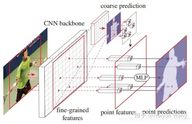
- 得到不确定点的位置以后,可以通过Bilinear插值得到对应的特征,对每个不确定点的使用一个MLP来进行单独进行细分预测【训练与预测有所区别】。
具体为:通过刚刚得到的不确定点所在图片的相对位置坐标来找到对应的特征点,将此点对应的特征向量与此点的粗糙预测结果合并,然后通过一个MLP进行细分预测。
- 代码如下:
##训练阶段
def forward(self, x, res2, out):
        """
        主要思路:
        通过 out(粗糙预测)计算出top N 个不稳定的像素点,针对每个不稳定像素点得到在res2(fine)
        和out(coarse)中对应的特征,组合N个不稳定像素点对应的fine和coarse得到rend,
        再通过mlp得到更准确的预测
        :param x: 表示输入图片的特征     eg.[2, 3, 768, 768]
        :param res2: 表示xception的第一层特征输出     eg.[2, 256, 192, 192]
        :param out: 表示经过级联空洞卷积提取的特征的粗糙预测    eg.[2, 19, 48, 48]
        :return: rend:更准确的预测,points:不确定像素点的位置
        """
        """
        1. Fine-grained features are interpolated from res2 for DeeplabV3
        2. During training we sample as many points as there are on a stride 16 feature map of the input
        3. To measure prediction uncertainty
           we use the same strategy during training and inference: the difference between the most
           confident and second most confident class probabilities.
        """
        if not self.training:
            return self.inference(x, res2, out)
		#获得不确定点的坐标
        points = sampling_points(out, x.shape[-1] // 16, self.k, self.beta) #out:[2, 19, 48, 48] || x:[2, 3, 768, 768] || points:[2, 48, 2]
		#根据不确定点的坐标,得到对应的粗糙预测
        coarse = point_sample(out, points, align_corners=False) #[2, 19, 48]
        #根据不确定点的坐标,得到对应的特征向量
        fine = point_sample(res2, points, align_corners=False)  #[2, 256, 48]
		#将粗糙预测与对应的特征向量合并
        feature_representation = torch.cat([coarse, fine], dim=1)   #[2, 275, 48]
		#使用MLP进行细分预测
        rend = self.mlp(feature_representation) #[2, 19, 48]

        return {"rend": rend, "points": points}

##推理阶段
@torch.no_grad()
    def inference(self, x, res2, out):
        """
        输入:
        x:[1, 3, 768, 768],表示输入图片的特征
        res2:[1, 256, 192, 192],表示xception的第一层特征输出
        out:[1, 19, 48, 48],表示经过级联空洞卷积提取的特征的粗糙预测
        输出:
        out:[1,19,768,768],表示最终图片的预测
        主要思路:
        通过 out计算出top N = 8096 个不稳定的像素点,针对每个不稳定像素点得到在res2(fine)
        和out(coarse)中对应的特征,组合8096个不稳定像素点对应的fine和coarse得到rend,
        再通过mlp得到更准确的预测,迭代至rend的尺寸大小等于输入图片的尺寸大小
        """
        """
        During inference, subdivision uses N=8096
        (i.e., the number of points in the stride 16 map of a 1024×2048 image)
        """
        num_points = 8096

        while out.shape[-1] != x.shape[-1]: #out:[1, 19, 48, 48], x:[1, 3, 768, 768]
        	#每一次预测均会扩大2倍像素,直至与原图像素大小一致
            out = F.interpolate(out, scale_factor=2, mode="bilinear", align_corners=True)   #out[1, 19, 48, 48]

            points_idx, points = sampling_points(out, num_points, training=self.training)   #points_idx:8096 || points:[1, 8096, 2]

            coarse = point_sample(out, points, align_corners=False) #coarse:[1, 19, 8096]   表示8096个不稳定像素点根据高级特征得出的对应的类别
            fine = point_sample(res2, points, align_corners=False)  #fine:[1, 256, 8096]    表示8096个不稳定像素点根据低级特征得出的对应类别

            feature_representation = torch.cat([coarse, fine], dim=1)   #[1, 275, 8096] 表示8096个不稳定像素点合并fine和coarse的特征

            rend = self.mlp(feature_representation) #[1, 19, 8096]

            B, C, H, W = out.shape  #first:[1, 19, 128, 256]
            points_idx = points_idx.unsqueeze(1).expand(-1, C, -1)  #[1, 19, 8096]
            out = (out.reshape(B, C, -1)
                      .scatter_(2, points_idx, rend)    #[1, 19, 32768]
                      .view(B, C, H, W))    #[1, 19, 128, 256]

        return {"fine": out}
3. Loss方面
- 由于有整体预测及细分点预测两部分,所以Loss也由这两部分加和而成
- 代码如下
class PointRendLoss(nn.CrossEntropyLoss):
    def __init__(self, aux=True, aux_weight=0.2, ignore_index=-1, **kwargs):
        super(PointRendLoss, self).__init__(ignore_index=ignore_index)
        self.aux = aux
        self.aux_weight = aux_weight
        self.ignore_index = ignore_index

    def forward(self, *inputs, **kwargs):
        result, gt = tuple(inputs)
        #result['res2']: [2, 256, 192, 192], 即xception的c1层提取到的特征
        #result['coarse']: [2, 19, 48, 48]
        #result['rend']: [2, 19, 48]
        #result['points']:[2, 48, 2]
        #gt:[2, 768, 768], 即图片对应的label

        #pred:[2, 19, 768, 768],将粗糙预测的插值到label大小
        pred = F.interpolate(result["coarse"], gt.shape[-2:], mode="bilinear", align_corners=True)

       	#整体像素点的交叉熵loss
        seg_loss = F.cross_entropy(pred, gt, ignore_index=self.ignore_index)

		#根据不确定点坐标获得不确定点对应的gt
        gt_points = point_sample(
            gt.float().unsqueeze(1),
            result["points"],
            mode="nearest",
            align_corners=False
        ).squeeze_(1).long()

        #不确定点的交叉熵loss
        points_loss = F.cross_entropy(result["rend"], gt_points, ignore_index=self.ignore_index)

		#整体+不确定点
        loss = seg_loss + points_loss

        return dict(loss=loss)
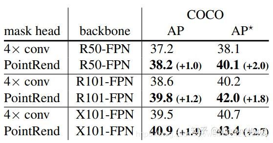
PointRend的实验效果:
- 关于实例分割:
- 在各种定量的评测中,PointRend均能提升1~2点的mask AP,而且展现出越强的backbone,越好的标注提升越高的特点。
- 实际视觉结果上,更是赏心悦目。同样的想法也可以用到语义分割任务中去,同样也可以取得提升。仅放题图一例,有兴趣的读者可以参见原文有更多清晰大图。

- 关于语义分割:个人将此模块应用于基础的语义分割模型,如Deeplabv3、Deeplabv3+ 等,效果均有1%以上的提升。但是视觉效果方面没有paper中那么明显。
总结:
简单总结一下,此paper是在常规方法,mask插值到原像素大小过程中,额外加入了对不好预测的点进行单独的细分处理,是个通用模块,对于精细分割领域这个思路可以借鉴。
另,有需要代码的小伙伴可以留下邮箱…