PMSM同步旋转坐标系下的数学模型及Simulink仿真

1.同步旋转坐标系下的数学模型

1.1 dq坐标系下的定子电压方程

1.2 dq坐标系下的定子磁链方程

1.3 定子电压方程变换式及等效电路

由上述两个方程，可以得到定子电压方程的新等式：

电压等效电路如下:

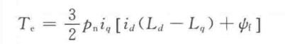
1.4 电磁转矩方程

1.5 相关重要关系式

其中，
$${\omega }_e表示电角速度，{\omega }_m表示机械角速度，n_p表示极对数，N_r表示电机转速，r/min，{\omega }_m单位为rad/s。$$

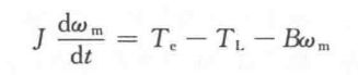
1.6 电机的机械运动方程

2.三相PMSM矢量控制仿真模型

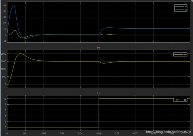
基于上述1.3的电压平衡方程，1.4的转矩方程，1.6的机械运动方程，可以构建矢量控制仿真模型，采用s-function形势，其中，Id,Iq,We为状态变量，仿真模型如下图所示：

仿真结果如下所示：

3.s-Function的运用

• 上述仿真过程中使用到了Simulink的S-function模块，S-Function可用来求解微分仿真，上述公式中，以Id，Iq,we作为微分方程的状态变量。
• S-Function的模板路径如下：…toolbox\simulink\blocks\sfuntmpl.m
• s-Function基于模板的编写过程，主要步骤为：
  步骤一：初始化设置，定义摄入输出个数、系统状态变量个数
  步骤二：相关参数设置以及微分仿真编写
  步骤三：设定系统输出变量

function [sys,x0,str,ts,simStateCompliance] = sfuntmpl(t,x,u,flag)
%SFUNTMPL General MATLAB S-Function Template
%   With MATLAB S-functions, you can define you own ordinary differential
%   equations (ODEs), discrete system equations, and/or just about
%   any type of algorithm to be used within a Simulink block diagram.
%
%   The general form of an MATLAB S-function syntax is:
%       [SYS,X0,STR,TS,SIMSTATECOMPLIANCE] = SFUNC(T,X,U,FLAG,P1,...,Pn)
%
%   What is returned by SFUNC at a given point in time, T, depends on the
%   value of the FLAG, the current state vector, X, and the current
%   input vector, U.
%
%   FLAG   RESULT             DESCRIPTION
%   -----  ------             --------------------------------------------
%   0      [SIZES,X0,STR,TS]  Initialization, return system sizes in SYS,
%                             initial state in X0, state ordering strings
%                             in STR, and sample times in TS.
%   1      DX                 Return continuous state derivatives in SYS.
%   2      DS                 Update discrete states SYS = X(n+1)
%   3      Y                  Return outputs in SYS.
%   4      TNEXT              Return next time hit for variable step sample
%                             time in SYS.
%   5                         Reserved for future (root finding).
%   9      []                 Termination, perform any cleanup SYS=[].
%
%
%   The state vectors, X and X0 consists of continuous states followed
%   by discrete states.
%
%   Optional parameters, P1,...,Pn can be provided to the S-function and
%   used during any FLAG operation.
%
%   When SFUNC is called with FLAG = 0, the following information
%   should be returned:
%
%      SYS(1) = Number of continuous states.
%      SYS(2) = Number of discrete states.
%      SYS(3) = Number of outputs.
%      SYS(4) = Number of inputs.
%               Any of the first four elements in SYS can be specified
%               as -1 indicating that they are dynamically sized. The
%               actual length for all other flags will be equal to the
%               length of the input, U.
%      SYS(5) = Reserved for root finding. Must be zero.
%      SYS(6) = Direct feedthrough flag (1=yes, 0=no). The s-function
%               has direct feedthrough if U is used during the FLAG=3
%               call. Setting this to 0 is akin to making a promise that
%               U will not be used during FLAG=3. If you break the promise
%               then unpredictable results will occur.
%      SYS(7) = Number of sample times. This is the number of rows in TS.
%
%
%      X0     = Initial state conditions or [] if no states.
%
%      STR    = State ordering strings which is generally specified as [].
%
%      TS     = An m-by-2 matrix containing the sample time
%               (period, offset) information. Where m = number of sample
%               times. The ordering of the sample times must be:
%
%               TS = [0      0,      : Continuous sample time.
%                     0      1,      : Continuous, but fixed in minor step
%                                      sample time.
%                     PERIOD OFFSET, : Discrete sample time where
%                                      PERIOD > 0 & OFFSET < PERIOD.
%                     -2     0];     : Variable step discrete sample time
%                                      where FLAG=4 is used to get time of
%                                      next hit.
%
%               There can be more than one sample time providing
%               they are ordered such that they are monotonically
%               increasing. Only the needed sample times should be
%               specified in TS. When specifying more than one
%               sample time, you must check for sample hits explicitly by
%               seeing if
%                  abs(round((T-OFFSET)/PERIOD) - (T-OFFSET)/PERIOD)
%               is within a specified tolerance, generally 1e-8. This
%               tolerance is dependent upon your model's sampling times
%               and simulation time.
%
%               You can also specify that the sample time of the S-function
%               is inherited from the driving block. For functions which
%               change during minor steps, this is done by
%               specifying SYS(7) = 1 and TS = [-1 0]. For functions which
%               are held during minor steps, this is done by specifying
%               SYS(7) = 1 and TS = [-1 1].
%
%      SIMSTATECOMPLIANCE = Specifices how to handle this block when saving and
%                           restoring the complete simulation state of the
%                           model. The allowed values are: 'DefaultSimState',
%                           'HasNoSimState' or 'DisallowSimState'. If this value
%                           is not speficified, then the block's compliance with
%                           simState feature is set to 'UknownSimState'.


%   Copyright 1990-2010 The MathWorks, Inc.

%
% The following outlines the general structure of an S-function.
%
switch flag,

  %%%%%%%%%%%%%%%%%%
  % Initialization %
  %%%%%%%%%%%%%%%%%%
  case 0,
    [sys,x0,str,ts,simStateCompliance]=mdlInitializeSizes;

  %%%%%%%%%%%%%%%
  % Derivatives %
  %%%%%%%%%%%%%%%
  case 1,
    sys=mdlDerivatives(t,x,u);

  %%%%%%%%%%
  % Update %
  %%%%%%%%%%
  case {2,4,9}
    sys=[];

  %%%%%%%%%%%
  % Outputs %
  %%%%%%%%%%%
  case 3,
    sys=mdlOutputs(t,x,u);

  %%%%%%%%%%%%%%%%%%%%
  % Unexpected flags %
  %%%%%%%%%%%%%%%%%%%%
  otherwise
    DAStudio.error('Simulink:blocks:unhandledFlag', num2str(flag));

end

% end sfuntmpl

%
%=============================================================================
% mdlInitializeSizes
% Return the sizes, initial conditions, and sample times for the S-function.
%=============================================================================
%
function [sys,x0,str,ts,simStateCompliance]=mdlInitializeSizes

%
% call simsizes for a sizes structure, fill it in and convert it to a
% sizes array.
%
% Note that in this example, the values are hard coded.  This is not a
% recommended practice as the characteristics of the block are typically
% defined by the S-function parameters.
%
sizes = simsizes;

sizes.NumContStates  = 3;
sizes.NumDiscStates  = 0;
sizes.NumOutputs     = 3;
sizes.NumInputs      = 3;
sizes.DirFeedthrough = 0;
sizes.NumSampleTimes = 1;   % at least one sample time is needed

sys = simsizes(sizes);

%
% initialize the initial conditions
%
x0  = [0;0;0];

%
% str is always an empty matrix
%
str = [];

%
% initialize the array of sample times
%
ts  = [0 0];

% Specify the block simStateCompliance. The allowed values are:
%    'UnknownSimState', < The default setting; warn and assume DefaultSimState
%    'DefaultSimState', < Same sim state as a built-in block
%    'HasNoSimState',   < No sim state
%    'DisallowSimState' < Error out when saving or restoring the model sim state
simStateCompliance = 'UnknownSimState';

% end mdlInitializeSizes

%
%=============================================================================
% mdlDerivatives
% Return the derivatives for the continuous states.
%=============================================================================
%
function sys=mdlDerivatives(t,x,u)

% % % 电机参数设置
R = 2.875;
Ld = 8.5e-3;
Lq = 8.5e-3;
Pn = 4;
Phi = 0.175;
J = 0.001;
B = 0.008;
% x(1)、 x(2)、x(3)分别对应系统的3个状态变量id,iq,wm
%u(1)、u(2)、u(3)分别对应ud,uq和TL

sys(1) = (1/Ld)*u(1) - (R/Ld)*x(1) + (Lq/Ld)*Pn*x(2)*x(3);
sys(2) = (1/Lq)*u(2) - (R/Lq)*x(2) - (Ld/Lq)* x(1)*x(3)*Pn - Phi*Pn*x(3)/Lq
sys(3) = (1/J)*(1.5*Pn*x(2)*((Ld-Lq)*x(1) + Phi) - u(3) - B*x(3))


% end mdlDerivatives

%
%=============================================================================
% mdlUpdate
% Handle discrete state updates, sample time hits, and major time step
% requirements.
%=============================================================================
%
function sys=mdlUpdate(t,x,u)

sys = [];

% end mdlUpdate

%
%=============================================================================
% mdlOutputs
% Return the block outputs.
%=============================================================================
%
function sys=mdlOutputs(t,x,u)
sys(1) = x(1);
sys(2) = x(2);
sys(3) = x(3);

% end mdlOutputs

%
%=============================================================================
% mdlGetTimeOfNextVarHit
% Return the time of the next hit for this block.  Note that the result is
% absolute time.  Note that this function is only used when you specify a
% variable discrete-time sample time [-2 0] in the sample time array in
% mdlInitializeSizes.
%=============================================================================
%
function sys=mdlGetTimeOfNextVarHit(t,x,u)

sampleTime = 1;    %  Example, set the next hit to be one second later.
sys = t + sampleTime;

% end mdlGetTimeOfNextVarHit

%
%=============================================================================
% mdlTerminate
% Perform any end of simulation tasks.
%=============================================================================
%
function sys=mdlTerminate(t,x,u)

sys = [];

% end mdlTerminate