pandas处理时序数据
快速浏览
- 时序的创建
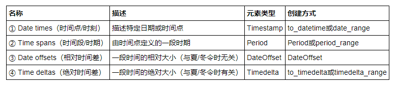
- 四类时间变量
- Date times(时间点/时刻)
- Date offsets(相对时间差)
- 时序的索引及属性
- 重采样
- 窗口函数rolling/expanding
- 练习
- Reference
时序的创建
四类时间变量
Date times(时间点/时刻)
Pandas在时间点建立的输入格式规定上给了很大的自由度,下面的语句都能正确建立同一时间点:
pd.to_datetime('2020.1.1')
pd.to_datetime('2020 1.1')
pd.to_datetime('2020 1 1')
pd.to_datetime('2020 1-1')
pd.to_datetime('2020-1 1')
pd.to_datetime('2020-1-1')
pd.to_datetime('2020/1/1')
pd.to_datetime('1.1.2020')
pd.to_datetime('1.1 2020')
pd.to_datetime('1 1 2020')
pd.to_datetime('1 1-2020')
pd.to_datetime('1-1 2020')
pd.to_datetime('1-1-2020')
pd.to_datetime('1/1/2020')
pd.to_datetime('20200101')
pd.to_datetime('2020.0101')
#下面的语句都会报错
#pd.to_datetime('2020\\1\\1')
#pd.to_datetime('2020`1`1')
#pd.to_datetime('2020.1 1')
#pd.to_datetime('1 1.2020')
语句会报错时可利用format参数强制匹配
pd.to_datetime('2020\\1\\1',format='%Y\\%m\\%d')
pd.to_datetime('2020`1`1',format='%Y`%m`%d')
pd.to_datetime('2020.1 1',format='%Y.%m %d')
pd.to_datetime('1 1.2020',format='%d %m.%Y')
使用列表可以将其转为时间点索引
print(pd.Series(range(2),index=pd.to_datetime(['2020/1/1','2020/1/2'])))
print(type(pd.to_datetime(['2020/1/1','2020/1/2'])))
2020-01-01    0
2020-01-02    1
dtype: int64
对于DataFrame而言,如果列已经按照时间顺序排好,则利用to_datetime可自动转换
df = pd.DataFrame({'year': [2020, 2020],'month': [1, 1], 'day': [1, 2]})
pd.to_datetime(df)
0   2020-01-01
1   2020-01-02
dtype: datetime64[ns]
Date times(时间点/时刻)Timestamp的精度远远不止day,可以最小到纳秒ns;同时,它带来范围的代价就是只有大约584年的时间点是可用.
print(pd.to_datetime('2020/1/1 00:00:00.123456789'))
print(pd.Timestamp.min)
print(pd.Timestamp.max)
2020-01-01 00:00:00.123456789
1677-09-21 00:12:43.145225
2262-04-11 23:47:16.854775807
date_range方法中start/end/periods(时间点个数)/freq(间隔方法)是该方法最重要的参数,给定了其中的3个,剩下的一个就会被确定。其中freq参数有许多选项(符号 D/B日/工作日 W周 M/Q/Y月/季/年末日 BM/BQ/BY月/季/年末工作日 MS/QS/YS月/季/年初日 BMS/BQS/BYS月/季/年初工作日 H小时 T分钟 S秒),更多选项可看此处
print(pd.date_range(start='2020/1/1',end='2020/1/10',periods=3))
print(pd.date_range(start='2020/1/1',end='2020/1/10',freq='D'))
print(pd.date_range(start='2020/1/1',periods=3,freq='D'))
print(pd.date_range(end='2020/1/3',periods=3,freq='D'))
print(pd.date_range(start='2020/1/1',periods=3,freq='T'))
print(pd.date_range(start='2020/1/1',periods=3,freq='M'))
print(pd.date_range(start='2020/1/1',periods=3,freq='BYS'))
DatetimeIndex(['2020-01-01 00:00:00', '2020-01-05 12:00:00',
               '2020-01-10 00:00:00'],
              dtype='datetime64[ns]', freq=None)
DatetimeIndex(['2020-01-01', '2020-01-02', '2020-01-03', '2020-01-04',
               '2020-01-05', '2020-01-06', '2020-01-07', '2020-01-08',
               '2020-01-09', '2020-01-10'],
              dtype='datetime64[ns]', freq='D')
DatetimeIndex(['2020-01-01', '2020-01-02', '2020-01-03'], dtype='datetime64[ns]', freq='D')
DatetimeIndex(['2020-01-01', '2020-01-02', '2020-01-03'], dtype='datetime64[ns]', freq='D')
DatetimeIndex(['2020-01-01 00:00:00', '2020-01-01 00:01:00',
               '2020-01-01 00:02:00'],
              dtype='datetime64[ns]', freq='T')
DatetimeIndex(['2020-01-31', '2020-02-29', '2020-03-31'], dtype='datetime64[ns]', freq='M')
DatetimeIndex(['2020-01-01', '2021-01-01', '2022-01-03'], dtype='datetime64[ns]', freq='BAS-JAN')
bdate_range是一个类似与date_range的方法,特点在于可以在自带的工作日间隔设置上,再选择weekmask参数和holidays参数。它的freq中有一个特殊的’C’/‘CBM’/'CBMS’选项,表示定制,需要联合weekmask参数和holidays参数使用。例如现在需要将工作日中的周一、周二、周五3天保留,并将部分holidays剔除
weekmask = 'Mon Tue Fri'
holidays = [pd.Timestamp('2020/1/%s'%i) for i in range(7,13)]
#注意holidays
pd.bdate_range(start='2020-1-1',end='2020-1-15',freq='C',weekmask=weekmask,holidays=holidays)
DatetimeIndex(['2020-01-03', '2020-01-06', '2020-01-13', '2020-01-14'], dtype='datetime64[ns]', freq='C')
Date offsets(相对时间差)
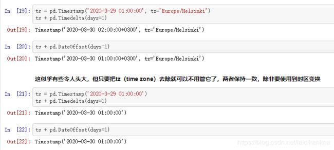
DataOffset与Timedelta的区别在于Timedelta绝对时间差的特点指无论是冬令时还是夏令时,增减1day都只计算24小时。而DataOffset相对时间差指,无论一天是23\24\25小时,增减1day都与当天相同的时间保持一致。
例如,英国当地时间 2020年03月29日,01:00:00 时钟向前调整 1 小时 变为 2020年03月29日,02:00:00,开始夏令时
DateOffset的可选参数包括years/months/weeks/days/hours/minutes/seconds
print(pd.Timestamp('2020-01-01') + pd.DateOffset(minutes=20) - pd.DateOffset(weeks=2))
2019-12-18 00:20:00
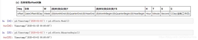
序列的offset操作
print(pd.Series(pd.offsets.BYearBegin(3).apply(i) for i in pd.date_range('20200101',periods=3,freq='Y')))
print(pd.date_range('20200101',periods=3,freq='Y') + pd.offsets.BYearBegin(3))
print(pd.Series(pd.offsets.CDay(3,weekmask='Wed Fri',holidays='2020010').apply(i)
                                  for i in pd.date_range('20200105',periods=3,freq='D')))
#pd.date_range('20200105',periods=3,freq='D')
#DatetimeIndex(['2020-01-05', '2020-01-06', '2020-01-07'], dtype='datetime64[ns]', freq='D')
0   2023-01-02
1   2024-01-01
2   2025-01-01
dtype: datetime64[ns]
DatetimeIndex(['2023-01-02', '2024-01-01', '2025-01-01'], dtype='datetime64[ns]', freq='A-DEC')
0   2020-01-15
1   2020-01-15
2   2020-01-15
dtype: datetime64[ns]
时序的索引及属性
索引切片几乎与pandas索引的规则完全一致。而且合法字符自动转换为时间点,也支持混合形态索引。
rng = pd.date_range('2020','2021', freq='W')
ts = pd.Series(np.random.randn(len(rng)), index=rng)
print(ts.head())
print(ts['2020-01-26'])
print(ts['2020-01-26':'20200306'])
print(ts['2020-7'])
print(ts['2011-1':'20200726'].head())
2020-01-05    1.101587
2020-01-12    0.344175
2020-01-19    0.521394
2020-01-26    0.535159
2020-02-02   -0.536123
Freq: W-SUN, dtype: float64
0.5351588314930403
2020-01-26    0.535159
2020-02-02   -0.536123
2020-02-09    0.109903
2020-02-16   -0.102390
2020-02-23   -0.524725
2020-03-01   -0.756281
Freq: W-SUN, dtype: float64
采用dt对象可以轻松获得关于时间的信息,对于datetime对象可以直接通过属性获取信息,利用strftime可重新修改时间格式。
#print(pd.Series(ts.index).dt.week)
#print(pd.Series(ts.index).dt.day)
print(pd.Series(ts.index).dt.strftime('%Y-间隔1-%m-间隔2-%d').head())
print(pd.Series(ts.index).dt.strftime('%Y年%m月%d日').head())
print(pd.date_range('2020','2021', freq='W').month)
0    2020-间隔1-01-间隔2-05
1    2020-间隔1-01-间隔2-12
2    2020-间隔1-01-间隔2-19
3    2020-间隔1-01-间隔2-26
4    2020-间隔1-02-间隔2-02
dtype: object
0    2020年01月05日
1    2020年01月12日
2    2020年01月19日
3    2020年01月26日
4    2020年02月02日
dtype: object
Int64Index([ 1,  1,  1,  1,  2,  2,  2,  2,  3,  3,  3,  3,  3,  4,  4,  4,  4,
             5,  5,  5,  5,  5,  6,  6,  6,  6,  7,  7,  7,  7,  8,  8,  8,  8,
             8,  9,  9,  9,  9, 10, 10, 10, 10, 11, 11, 11, 11, 11, 12, 12, 12,
            12],
           dtype='int64')
重采样
所谓重采样,就是指resample函数,它可以看做时序版本的groupby函数。采样频率一般设置为上面提到的offset字符,
print(pd.date_range('1/1/2020', freq='S', periods=1000))
df_r = pd.DataFrame(np.random.randn(1000, 3),index=pd.date_range('1/1/2020', freq='S', periods=1000),
                  columns=['A', 'B', 'C'])
r = df_r.resample('3min')
print(r.sum())
DatetimeIndex(['2020-01-01 00:00:00', '2020-01-01 00:00:01',
               '2020-01-01 00:00:02', '2020-01-01 00:00:03',
               '2020-01-01 00:00:04', '2020-01-01 00:00:05',
               '2020-01-01 00:00:06', '2020-01-01 00:00:07',
               '2020-01-01 00:00:08', '2020-01-01 00:00:09',
               ...
               '2020-01-01 00:16:30', '2020-01-01 00:16:31',
               '2020-01-01 00:16:32', '2020-01-01 00:16:33',
               '2020-01-01 00:16:34', '2020-01-01 00:16:35',
               '2020-01-01 00:16:36', '2020-01-01 00:16:37',
               '2020-01-01 00:16:38', '2020-01-01 00:16:39'],
              dtype='datetime64[ns]', length=1000, freq='S')
                            A          B          C
2020-01-01 00:00:00 -6.214172  15.056536  -2.040001
2020-01-01 00:03:00 -0.974375  -5.857030 -10.369295
2020-01-01 00:06:00  1.836822  17.165221   9.111447
2020-01-01 00:09:00  2.030140   4.314473  14.528695
2020-01-01 00:12:00  7.339233   5.753052 -24.641334
2020-01-01 00:15:00 -8.736690  -0.122362  -2.023157
df_r2 = pd.DataFrame(np.random.randn(200, 3),index=pd.date_range('1/1/2020', freq='D', periods=200),
                  columns=['A', 'B', 'C'])
r = df_r2.resample('CBMS')
print(r.sum())
                   A          B         C
2020-01-01  1.518244  -0.743317 -3.515077
2020-02-03  1.378320   4.415827 -1.629024
2020-03-02 -0.705835  10.281621 -5.257010
2020-04-01  1.783766  -3.383655  2.103400
2020-05-01  4.551639   0.141568  5.081334
2020-06-01  2.434142  -1.549992 -0.175485
2020-07-01  0.569179  -2.901138 -4.751556
采样聚合
r = df_r.resample('3T')
print(r['A'].mean())
print(r['A'].agg([np.sum, np.mean, np.std]))
#类似地,可以使用函数/lambda表达式
print(r.agg({'A': np.sum,'B': lambda x: max(x)-min(x)}))
2020-01-01 00:00:00   -0.034523
2020-01-01 00:03:00   -0.005413
2020-01-01 00:06:00    0.010205
2020-01-01 00:09:00    0.011279
2020-01-01 00:12:00    0.040774
2020-01-01 00:15:00   -0.087367
Freq: 3T, Name: A, dtype: float64
                          sum      mean       std
2020-01-01 00:00:00 -6.214172 -0.034523  1.083538
2020-01-01 00:03:00 -0.974375 -0.005413  0.994005
2020-01-01 00:06:00  1.836822  0.010205  0.970560
2020-01-01 00:09:00  2.030140  0.011279  1.017799
2020-01-01 00:12:00  7.339233  0.040774  1.068230
2020-01-01 00:15:00 -8.736690 -0.087367  0.969861
                            A         B
2020-01-01 00:00:00 -6.214172  5.676805
2020-01-01 00:03:00 -0.974375  5.332746
2020-01-01 00:06:00  1.836822  5.207914
2020-01-01 00:09:00  2.030140  5.258446
2020-01-01 00:12:00  7.339233  5.680593
2020-01-01 00:15:00 -8.736690  5.490354
采样组的迭代和groupby迭代完全类似,对于每一个组都可以分别做相应操作
small = pd.Series(range(6),index=pd.to_datetime(['2020-01-01 00:00:00', '2020-01-01 00:30:00'
                                                 , '2020-01-01 00:31:00','2020-01-01 01:00:00'
                                                 ,'2020-01-01 03:00:00','2020-01-01 03:05:00']))
resampled = small.resample('H')
for name, group in resampled:
    print("Group: ", name)
    print("-" * 27)
    print(group, end="\n\n")
Group:  2020-01-01 00:00:00
---------------------------
2020-01-01 00:00:00    0
2020-01-01 00:30:00    1
2020-01-01 00:31:00    2
dtype: int64

Group:  2020-01-01 01:00:00
---------------------------
2020-01-01 01:00:00    3
dtype: int64

Group:  2020-01-01 02:00:00
---------------------------
Series([], dtype: int64)

Group:  2020-01-01 03:00:00
---------------------------
2020-01-01 03:00:00    4
2020-01-01 03:05:00    5
dtype: int64
窗口函数rolling/expanding
s = pd.Series(np.random.randn(1000),index=pd.date_range('1/1/2020', periods=1000))
print(s)
2020-01-01    0.404380
2020-01-02   -0.211402
2020-01-03   -1.398175
2020-01-04    1.018577
2020-01-05    0.894150
                ...
2022-09-22    0.132534
2022-09-23    0.606834
2022-09-24   -0.598215
2022-09-25   -0.127116
2022-09-26   -1.714029
Freq: D, Length: 1000, dtype: float64
rolling方法,就是规定一个窗口(min_periods参数是指需要的非缺失数据点数量阀值),它和groupby对象一样,本身不会进行操作,需要配合聚合函数才能计算结果。count/sum/mean/median/min/max/std/var/skew/kurt/quantile/cov/corr都是常用的聚合函数。使用apply聚合时,只需记住传入的是window大小的Series,输出的必须是标量即可。
基于时间的rolling可选closed=‘right’(默认)‘left’‘both’'neither’参数,决定端点的包含情况。
print(s.rolling(window=50))
print(s.rolling(window=50).mean())
print(s.rolling(window=50,min_periods=3).mean().head())
print(s.rolling(window=50,min_periods=3).apply(lambda x:x.std()/x.mean()).head())#计算变异系数
print(s.rolling('15D').mean().head())
print(s.rolling('15D', closed='right').sum().head())
Rolling [window=50,center=False,axis=0]
2020-01-01         NaN
2020-01-02         NaN
2020-01-03         NaN
2020-01-04         NaN
2020-01-05         NaN
                ...
2022-09-22   -0.059734
2022-09-23   -0.059340
2022-09-24   -0.086238
2022-09-25   -0.062391
2022-09-26   -0.068321
Freq: D, Length: 1000, dtype: float64
2020-01-01         NaN
2020-01-02         NaN
2020-01-03   -0.401732
2020-01-04   -0.046655
2020-01-05    0.141506
Freq: D, dtype: float64
2020-01-01          NaN
2020-01-02          NaN
2020-01-03    -2.280690
2020-01-04   -22.108891
2020-01-05     6.977926
Freq: D, dtype: float64
2020-01-01    0.404380
2020-01-02    0.096489
2020-01-03   -0.401732
2020-01-04   -0.046655
2020-01-05    0.141506
Freq: D, dtype: float64
2020-01-01    0.404380
2020-01-02    0.192979
2020-01-03   -1.205196
2020-01-04   -0.186619
2020-01-05    0.707531
Freq: D, dtype: float64
普通的expanding函数等价与rolling(window=len(s),min_periods=1),是对序列的累计计算。apply方法也是同样可用的,cumsum/cumprod/cummax/cummin都是特殊expanding累计计算方法。
print(s.rolling(window=len(s),min_periods=1).sum().head())
print(s.expanding().sum().head())
print(s.expanding().apply(lambda x:sum(x)).head())
print(s.cumsum().head())
2020-01-01    0.404380
2020-01-02    0.192979
2020-01-03   -1.205196
2020-01-04   -0.186619
2020-01-05    0.707531
Freq: D, dtype: float64
2020-01-01    0.404380
2020-01-02    0.192979
2020-01-03   -1.205196
2020-01-04   -0.186619
2020-01-05    0.707531
Freq: D, dtype: float64
2020-01-01    0.404380
2020-01-02    0.192979
2020-01-03   -1.205196
2020-01-04   -0.186619
2020-01-05    0.707531
Freq: D, dtype: float64
2020-01-01    0.404380
2020-01-02    0.192979
2020-01-03   -1.205196
2020-01-04   -0.186619
2020-01-05    0.707531
Freq: D, dtype: float64
shift/diff/pct_change都是涉及到了元素关系
①shift是指序列索引不变,但值向后移动
②diff是指前后元素的差,period参数表示间隔,默认为1,并且可以为负
③pct_change是值前后元素的变化百分比,period参数与diff类似

练习
【练习一】 现有一份关于某超市牛奶销售额的时间序列数据time_series_one.csv,请完成下列问题:
(a)销售额出现最大值的是星期几?(提示:利用dayofweek函数)
df = pd.read_csv('data/time_series_one.csv', parse_dates=['日期'])
df['日期'].dt.dayofweek[df['销售额'].idxmax()]
6
(b)计算除去春节、国庆、五一节假日的月度销售总额
holiday = pd.date_range(start='20170501', end='20170503').append(
          pd.date_range(start='20171001', end='20171007')).append(
          pd.date_range(start='20180215', end='20180221')).append(
          pd.date_range(start='20180501', end='20180503')).append(
          pd.date_range(start='20181001', end='20181007')).append(
          pd.date_range(start='20190204', end='20190224')).append(
          pd.date_range(start='20190501', end='20190503')).append(
          pd.date_range(start='20191001', end='20191007'))
result = df[~df['日期'].isin(holiday)].set_index('日期').resample('MS').sum()
result
(c)按季度计算周末(周六和周日)的销量总额
result = df[df['日期'].dt.dayofweek.isin([5,6])].set_index('日期').resample('QS').sum()
result
(d)从最后一天开始算起,跳过周六和周一,以5天为一个时间单位向前计算销售总和
df_temp = df[~df['日期'].dt.dayofweek.isin([5,6])].set_index('日期').iloc[::-1]
L_temp,date_temp = [],[0]*df_temp.shape[0]
for i in range(df_temp.shape[0]//5):
    L_temp.extend([i]*5)
L_temp.extend([df_temp.shape[0]//5]*(df_temp.shape[0]-df_temp.shape[0]//5*5))
date_temp = pd.Series([i%5==0 for i in range(df_temp.shape[0])])
df_temp['num'] = L_temp
result = pd.DataFrame({'5天总额':df_temp.groupby('num')['销售额'].sum().values},
                       index=df_temp.reset_index()[date_temp]['日期']).iloc[::-1]
result
(e)假设现在发现数据有误,所有同一周里的周一与周五的销售额记录颠倒了,请计算2018年中每月第一个周一的销售额(如果该周没有周一或周五的记录就保持不动)
from datetime import datetime
df_temp = df.copy()
df_fri = df.shift(4)[df.shift(4)['日期'].dt.dayofweek==1]['销售额']
df_mon = df.shift(-4)[df.shift(-4)['日期'].dt.dayofweek==5]['销售额']
df_temp.loc[df_fri.index,['销售额']] = df_fri
df_temp.loc[df_mon.index,['销售额']] = df_mon
df_temp.loc[df_temp[df_temp['日期'].dt.year==2018]['日期'][
        df_temp[df_temp['日期'].dt.year==2018]['日期'].apply(
        lambda x:True if datetime.strptime(str(x).split()[0],'%Y-%m-%d').weekday() == 0
        and 1 <= datetime.strptime(str(x).split()[0],'%Y-%m-%d').day <= 7 else False)].index,:]
【练习二】 继续使用上一题的数据,请完成下列问题:
(a)以50天为窗口计算滑窗均值和滑窗最大值(min_periods设为1)
df = pd.read_csv('data/time_series_one.csv',index_col='日期',parse_dates=['日期'])
df['销售额'].rolling(window=50,min_periods=1).mean().head()
df['销售额'].rolling(window=50,min_periods=1).max().head()
(b)现在有如下规则:若当天销售额超过向前5天的均值,则记为1,否则记为0,请给出2018年相应的计算结果
def f(x):
    if len(x) == 6:
        return 1 if x[-1]>np.mean(x[:-1]) else 0
    else:
        return 0
result_b = df.loc[pd.date_range(start='20171227',end='20181231'),:].rolling(
                                                    window=6,min_periods=1).agg(f)[5:].head()
result_b.head()
(c)将©中的“向前5天”改为“向前非周末5天”,请再次计算结果
def f(x):
    if len(x) == 8:
        return 1 if x[-1]>np.mean(x[:-1][pd.Series([
            False if i in [5,6] else True for i in x[:-1].index.dayofweek],index=x[:-1].index)]) else 0
    else:
        return 0
result_c = df.loc[pd.date_range(start='20171225',end='20181231'),:].rolling(
                                    window=8,min_periods=1).agg(f)[7:].head()
result_c.head()
比较巧合,与(b)的结果一样
Reference
- pandas官网
- Joyful-Pandas