Tree methods such as CART (classification and regression trees) can be used as alternatives to logistic regression. It is a way that can be used to show the probability of being in any hierarchical group. The following is a compilation of many of the key R packages that cover trees and forests. The goal here is to simply give some brief examples on a few approaches on growing trees and, in particular, the visualization of the trees. These packages include classification and regression trees, graphing and visualization, ensemble learning using random forests, as well as evolutionary learning trees. There are a wide array of package in R that handle decision trees including trees for longitudinal studies. I have found that when using several combinations of these packages simultaneously that some of the function begin to fail to work.
The concept of trees and forests can be applied in many different settings and is often seen in machine learning and data mining settings or other settings where there is a significant amount of data. The examples below are by no means comprehensive and exhaustive. However, there are several examples given using different datasets and a variety of R packages. The first example uses some data obtain from the Harvard Dataverse Network. For reference these data can be obtained from http://dvn.iq.harvard.edu/dvn/. The study was recently released on April 22nd, 2013 and the raw data as well as the documentation is available on the Dataverse web site and the study ID is hdl:1902.1/21235. The other examples use data that are shipped with the R packages.
rpart
This package includes several example sets of data that can be used for recursive partitioning and regression trees. Categorical or continuous variables can be used depending on whether one wants classification trees or regression trees. This package as well at the tree package are probably the two go-to packages for trees. However, care should be taken as the tree package and the rpart package can produce very different results.
01.
library(rpart)
02.
raw.orig < - read.csv(file="c:\\rsei212_chemical.txt", header=T, sep="\t")
03.
04.
# Keep the dataset small and tidy
05.
# The Dataverse: hdl:1902.1/21235
06.
raw = subset(raw.orig, select=c("Metal","OTW","AirDecay","Koc"))
07.
08.
row.names(raw) = raw.orig$CASNumber
09.
raw = na.omit(raw);
10.
11.
frmla = Metal ~ OTW + AirDecay + Koc
12.
13.
# Metal: Core Metal (CM); Metal (M); Non-Metal (NM); Core Non-Metal (CNM)
14.
15.
fit = rpart(frmla, method="class", data=raw)
16.
17.
printcp(fit) # display the results
18.
plotcp(fit) # visualize cross-validation results
19.
summary(fit) # detailed summary of splits
20.
21.
# plot tree
22.
plot(fit, uniform=TRUE, main="Classification Tree for Chemicals")
23.
text(fit, use.n=TRUE, all=TRUE, cex=.8)
24.
25.
# tabulate some of the data
26.
table(subset(raw, Koc>=190.5)$Metal)
tree
This is the primary R package for classification and regression trees. It has functions to prune the tree as well as general plotting functions and the mis-classifications (total loss). The output from tree can be easier to compare to the General Linear Model (GLM) and General Additive Model (GAM) alternatives.
1.
###############
2.
# TREE package
3.
library(tree)
4.
5.
tr = tree(frmla, data=raw)
6.
summary(tr)
7.
plot(tr); text(tr)
party
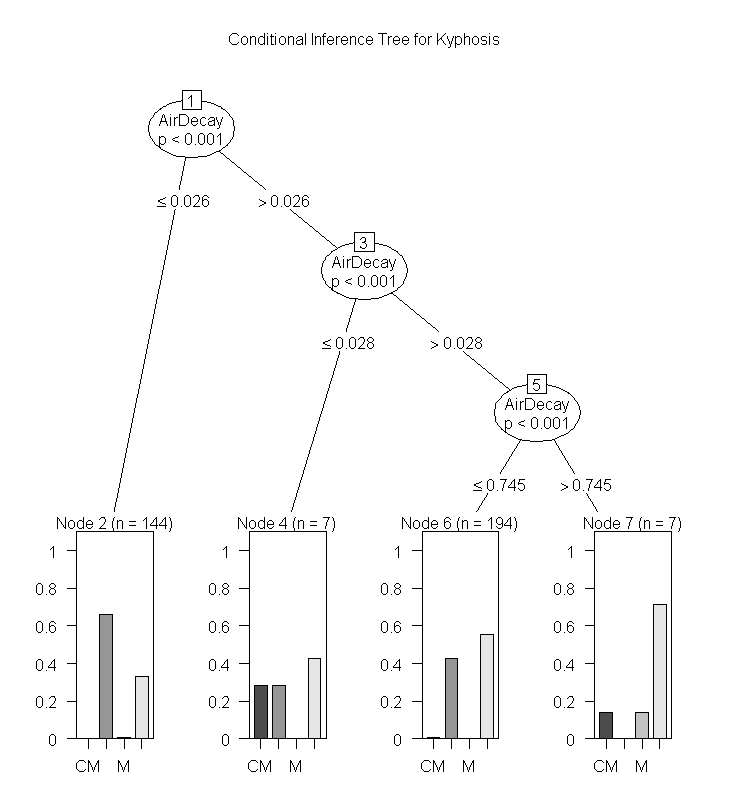
This is another package for recursive partitioning. One of the key functions in this package is ctree. As the package documention indicates it can be used for continuous, censored, ordered, nominal and multivariate response variable in a conditional inference framework. The party package also implements recursive partitioning for survival data.
01.
###############
02.
# PARTY package
03.
library(party)
04.
05.
(ct = ctree(frmla, data = raw))
06.
plot(ct, main="Conditional Inference Tree")
07.
08.
#Table of prediction errors
09.
table(predict(ct), raw$Metal)
10.
11.
# Estimated class probabilities
12.
tr.pred = predict(ct, newdata=raw, type="prob")
maptree
maptree is a very good at graphing, pruning data from hierarchical clustering, and CART models. The trees produced by this package tend to be better labeled and higher quality and the stock plots from rpart.
01.
###############
02.
# MAPTREE
03.
library(maptree)
04.
library(cluster)
05.
draw.tree( clip.rpart (rpart ( raw), best=7),
06.
nodeinfo=TRUE, units="species",
07.
cases="cells", digits=0)
08.
a = agnes ( raw[2:4], method="ward" )
09.
names(a)
10.
a$diss
11.
b = kgs (a, a$diss, maxclust=20)
12.
13.
plot(names(b), b, xlab="# clusters", ylab="penalty", type="n")
14.
xloc = names(b)[b==min(b)]
15.
yloc = min(b)
16.
ngon(c(xloc,yloc+.75,10, "dark green"), angle=180, n=3)
17.
apply(cbind(names(b), b, 3, 'blue'), 1, ngon, 4) # cbind(x,y,size,color)
partykit
This contains a re-implementation of the ctree function and it provides some very good graphing and visualization for tree models. It is similar to the party package. The example below uses data from airquality dataset and the famous species data available in R and can be found in the documentation.
1.
"http://statistical-research.com/wp-content/uploads/2012/12/species.png">![</code]()
"Species Decision Tree" src="http://statistical-research.com/wp-content/uploads/2012/12/species.png" width="437" height="472"/> "http://statistical-research.com/wp-content/uploads/2012/12/airqualityOzone.png">![</code]()
"Ozone Air Quality Decision Tree" src="http://statistical-research.com/wp-content/uploads/2012/12/airqualityOzone.png"width="437" height="472" />evtree
This package uses evolutionary algorithms. The idea behind this approach is that is will reduce the a priori bias. I have seen trees of this sort in the area of environmental research, bioinformatics, systematics, and marine biology. Though there are many other areas than that of phylogentics.
1.
###############
2.
## EVTREE (Evoluationary Learning)
3.
library(evtree)
4.
5.
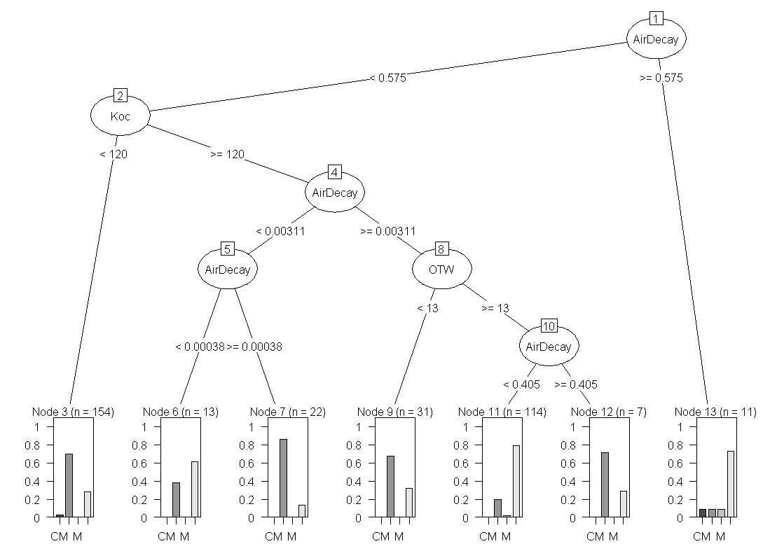
ev.raw = evtree(frmla, data=raw)
6.
plot(ev.raw)
7.
table(predict(ev.raw), raw$Metal)
8.
1-mean(predict(ev.raw) == raw$Metal)
randomForest
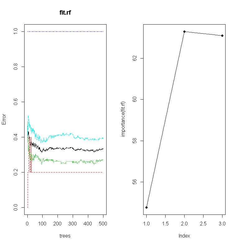
Random forests are very good in that it is an ensemble learning method used for classification and regression. It uses multiple models for better performance that just using a single tree model. In addition because many sample are selected in the process a measure of variable importance can be obtain and this approach can be used for model selection and can be particularly useful when forward/backward stepwise selection is not appropriate and when working with an extremely high number of candidate variables that need to be reduced.
01.
##################
02.
## randomForest
03.
library(randomForest)
04.
fit.rf = randomForest(frmla, data=raw)
05.
print(fit.rf)
06.
importance(fit.rf)
07.
plot(fit.rf)
08.
plot( importance(fit.rf), lty=2, pch=16)
09.
lines(importance(fit.rf))
10.
imp = importance(fit.rf)
11.
impvar = rownames(imp)[order(imp[, 1], decreasing=TRUE)]
12.
op = par(mfrow=c(1, 3))
13.
for (i in seq_along(impvar)) {
14.
partialPlot(fit.rf, raw, impvar[i], xlab=impvar[i],
15.
main=paste("Partial Dependence on", impvar[i]),
16.
ylim=c(0, 1))
17.
}
| >importance(rf1) | ||
| %IncMSE | IncNodePurity | |
| x1 | 30.30146 | 8657.963 |
| x2 | 7.739163 | 3675.853 |
| x3 | 0.586905 | 240.275 |
| x4 | -0.82209 | 381.6304 |
| x5 | 0.583622 | 253.3885 |
varSelRF
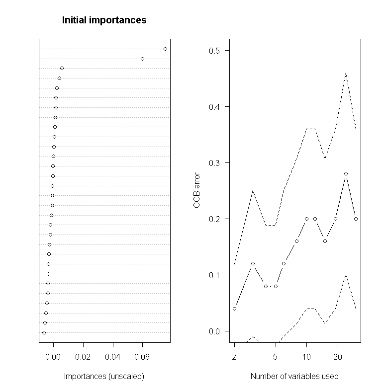
This can be used for further variable selection procedure using random forests. It implements both backward stepwise elimination as well as selection based on the importance spectrum. This data uses randomly generated data so the correlation matrix can set so that the first variable is strongly correlated and the other variables are less so.
01.
##################
02.
## varSelRF package
03.
library(varSelRF)
04.
x = matrix(rnorm(25 * 30), ncol = 30)
05.
x[1:10, 1:2] = x[1:10, 1:2] + 2
06.
cl = factor(c(rep("A", 10), rep("B", 15)))
07.
rf.vs1 = varSelRF(x, cl, ntree = 200, ntreeIterat = 100,
08.
vars.drop.frac = 0.2)
09.
10.
rf.vs1
11.
plot(rf.vs1)
12.
13.
## Example of importance function show that forcing x1 to be the most important
14.
## while create secondary variables that is related to x1.
15.
x1=rnorm(500)
16.
x2=rnorm(500,x1,1)
17.
y=runif(1,1,10)*x1+rnorm(500,0,.5)
18.
my.df=data.frame(y,x1,x2,x3=rnorm(500),x4=rnorm(500),x5=rnorm(500))
19.
rf1 = randomForest(y~., data=my.df, mtry=2, ntree=50, importance=TRUE)
20.
importance(rf1)
21.
cor(my.df)
oblique.tree
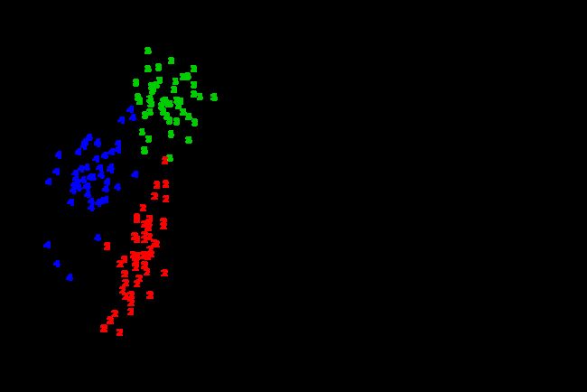
This package grows an oblique decision tree (a general form of the axis-parallel tree). This example uses the crab dataset (morphological measurements on Leptograpsus crabs) available in R as a stock dataset to grow the oblique tree.
01.
###############
02.
## OBLIQUE.TREE
03.
library(oblique.tree)
04.
05.
aug.crabs.data = data.frame( g=factor(rep(1:4,each=50)),
06.
predict(princomp(crabs[,4:8]))[,2:3])
07.
plot(aug.crabs.data[,-1],type="n")
08.
text( aug.crabs.data[,-1], col=as.numeric(aug.crabs.data[,1]), labels=as.numeric(aug.crabs.data[,1]))
09.
ob.tree = oblique.tree(formula = g~.,
10.
data = aug.crabs.data,
11.
oblique.splits = "only")
12.
plot(ob.tree);text(ob.tree)
CORElearn
This is a great package that contain many different machine learning algorithms and functions. It include trees, forests, naive Bayes, locally weighted regression, among others.
01.
##################
02.
## CORElearn
03.
04.
library(CORElearn)
05.
## Random Forests
06.
fit.rand.forest = CoreModel(frmla, data=raw, model="rf", selectionEstimator="MDL", minNodeWeightRF=5, rfNoTrees=100)
07.
plot(fit.rand.forest)
08.
09.
## decision tree with naive Bayes in the leaves
10.
fit.dt = CoreModel(frmla, raw, model="tree", modelType=4)
11.
plot(fit.dt, raw)
12.
13.
airquality.sub = subset(airquality, !is.na(airquality$Ozone))
14.
fit.rt = CoreModel(Ozone~., airquality.sub, model="regTree", modelTypeReg=1)
15.
summary(fit.rt)
16.
plot(fit.rt, airquality.sub, graphType="prototypes")
17.
18.
pred = predict(fit.rt, airquality.sub)
19.
print(pred)
20.
plot(pred)
longRPart
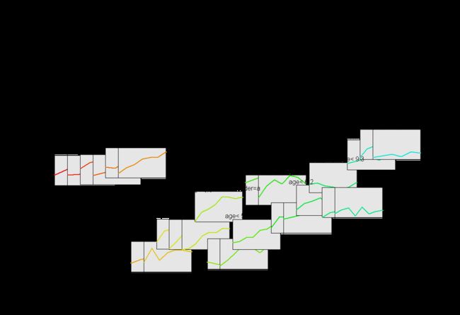
This provides an implementation for recursive partitioning for longitudinal data. It uses the rules from rpart and the mixed effects models from nlme to grow regression trees. This can be a little resource intensive on some slower computers.
1.
##################
2.
##longRPart
3.
library(longRPart)
4.
5.
data(pbkphData)
6.
pbkphData$Time=as.factor(pbkphData$Time)
7.
long.tree = longRPart(pbkph~Time,~age+gender,~1|Subject,pbkphData,R=corExp(form=~time))
8.
lrpTreePlot(long.tree, use.n=TRE, place="bottomright")
REEMtree
This package is useful for longitudinal studies where random effects exist. This example uses the pbkphData dataset available in the longRPart package.
01.
##################
02.
## REEMtree Random Effects for Longitudinal Data
03.
library(REEMtree)
04.
pbkphData.sub = subset(pbkphData, !is.na(pbkphData$pbkph))
05.
reem.tree = REEMtree(pbkph~Time, data=pbkphData.sub, random=~1|Subject)
06.
plot(reem.tree)
07.
ranef(reem.tree) #random effects
08.
09.
reem.tree = REEMtree(pbkph~Time, data=pbkphData.sub, random=~1|Subject,
10.
correlation=corAR1())
11.
plot(reem.tree)


