CS224N Assignment 1: Exploring Word Vectors (25 Points)
CS224N Assignment 1: Exploring Word Vectors (25 Points)
最近想自学一下自然语言处理,网上找了 Stanford CS224N 的网课,顺藤摸瓜找了点作业题来坐坐。下载链接:斯坦福 cs224n 课程网站
Part 1: Count-Based Word Vectors (10 points)
之前导入软件包如果出现问题的话,根据所需的包名一个个导入就可以了,推荐使用国内镜像网站,在 Win+R 输入 cmd ,那个窗口输入:
pip install 包名 -i https://pypi.tuna.tsinghua.edu.cn/simple
Question 1.1: Implement distinct_words [code] (2 points)
这道题目的让你获取 单词列表 的列表 中不同单词的,其实就是让你熟悉一下使用 python 。
这里使用集合这个数据结构来实现(集合是 Hash 表存储结构,读取起来更快)。然后每次循环在旧集合与新列表之间取并集即可:
## Question 1.1: Implement distinct_words [code] (2 points)
def distinct_words(corpus):
    """ Determine a list of distinct words for the corpus.
        Params:
            corpus (list of list of strings): corpus of documents
        Return:
            corpus_words (list of strings): list of distinct words across the corpus, sorted (using python 'sorted' function)
            num_corpus_words (integer): number of distinct words across the corpus
    """
    corpus_words = []
    num_corpus_words = -1

    # ------------------
    # Write your implementation here.
    corpus_words = set()
    for item in corpus:
        words = set(item)
        corpus_words = corpus_words | words
    num_corpus_words = len(corpus_words)
    corpus_words = sorted(list(corpus_words))
    # ------------------

    return corpus_words, num_corpus_words
测试一下:
>>> --------------------------------------------------------------------------------
	Passed All Tests!
	--------------------------------------------------------------------------------
Question 1.2: Implement compute_co_occurrence_matrix [code] (3 points)
第二个问题是构建一个邻接矩阵。首先先看它需要返回的两个东西:
- 第一个
word2ind是由字符作为key,这个字符在之前第一小问返回的列表中的索引作为val的一个字典结构。根据这个结构,使我们能够在 O ( 1 ) O(1) O(1) 的时间复杂度下获得矩阵的位置。关于怎么创建全 0 0 0 矩阵,见底下代码 - 第二个
M是一个矩阵,这个矩阵包含了信息:出现在这个词左右的,是什么词。我们只需要对当前字符串进行一次遍历,在每次遍历的时候,注意window这个变量,我们需要统计这个词 ± w i n d o w ±window ±window 这个变量周围的所有单词。
先回顾一下课堂上讲的知识:为什么这个窗口是可行的:这个窗口就是这个单词出现的上下文,因此出现在类似窗口(也即类似上下文)中的两个单词,他们的词意一般是类似的,因此类似意思的两个单词会聚类在一起。
如果忘了 numpy 的使用方法,见:数据可视化学习笔记【一】(numpy包)。
实现代码如下:
## Question 1.2: Implement compute_co_occurrence_matrix [code] (3 points)
def compute_co_occurrence_matrix(corpus, window_size=4):
    """ Compute co-occurrence matrix for the given corpus and window_size (default of 4).

        Note: Each word in a document should be at the center of a window. Words near edges will have a smaller
              number of co-occurring words.

              For example, if we take the document " All that glitters is not gold " with window size of 4,
              "All" will co-occur with "", "that", "glitters", "is", and "not".

        Params:
            corpus (list of list of strings): corpus of documents
            window_size (int): size of context window
        Return:
            M (a symmetric numpy matrix of shape (number of unique words in the corpus , number of unique words in the corpus)):
                Co-occurence matrix of word counts.
                The ordering of the words in the rows/columns should be the same as the ordering of the words given by the distinct_words function.
            word2Ind (dict): dictionary that maps word to index (i.e. row/column number) for matrix M.
    """
    words, num_words = distinct_words(corpus)
    M = None
    word2Ind = {}

    # ------------------
    # Write your implementation here.
    i = 0
    for key in words:
        word2Ind[key] = i
        i += 1
    M = np.zeros((num_words, num_words))
    for sentence in corpus:
        for i, word in enumerate(sentence):
            for j in range(i - window_size, i + window_size + 1):
                if j < 0 or j >= len(sentence):
                    continue
                if j != i:
                    M[word2Ind[word], word2Ind[sentence[j]]] += 1
    # ------------------

    return M, word2Ind
执行:
>>> --------------------------------------------------------------------------------
	Passed All Tests!
	--------------------------------------------------------------------------------
Question 1.3: Implement reduce_to_k_dim [code] (1 point)
这题就是导包,进行 SVD 分解( M = U Σ V T M = U\Sigma V^{T} M=UΣVT 其中 U , V U,V U,V 都是酉矩阵, Σ \Sigma Σ 为对角矩阵,且 r a n k ( Σ ) = r a n k ( M ) rank(\Sigma)=rank(M) rank(Σ)=rank(M)),保留奇异值前 k 大的值,然后得到一个降维的矩阵 U Σ U\Sigma UΣ 。
原来那个 10 ∗ 10 10*10 10∗10 的矩阵被降为一个 10 ∗ 2 10*2 10∗2 的矩阵了。
[0.65480209 		0.78322112]
[5.20200324e-01 		-1.56599893e-15]
[0.70564718 		-0.48405727]
[0.70564718 		0.48405727]
[1.02780472e+00 		1.01204090e-15]
[0.65480209 		-0.78322112]
[0.38225849 		-0.656224  ]
[0.38225849 		0.656224  ]
[1.39420808 		1.06179274]
[1.39420808 		-1.06179274]
为什么要进行这部操作呢?之前课上说到:人是一个三维生物,很难想象到一个高维空间,比如之前那个 10 ∗ 10 10*10 10∗10 矩阵所表示的一个 10 10 10 维空间显然超过了人类的理解范围,因此将其降维。(同时有一个小小的推测,这里相当于加上了一个小扰动,是不是为了防止模型会产生过拟合?)
代码实现如下:
def reduce_to_k_dim(M, k=2):
    """ Reduce a co-occurence count matrix of dimensionality (num_corpus_words, num_corpus_words)
        to a matrix of dimensionality (num_corpus_words, k) using the following SVD function from Scikit-Learn:
            - http://scikit-learn.org/stable/modules/generated/sklearn.decomposition.TruncatedSVD.html

        Params:
            M (numpy matrix of shape (number of unique words in the corpus , number of unique words in the corpus)): co-occurence matrix of word counts
            k (int): embedding size of each word after dimension reduction
        Return:
            M_reduced (numpy matrix of shape (number of corpus words, k)): matrix of k-dimensioal word embeddings.
                    In terms of the SVD from math class, this actually returns U * S
    """
    n_iters = 10     # Use this parameter in your call to `TruncatedSVD`
    M_reduced = None
    print("Running Truncated SVD over %i words..." % (M.shape[0]))

        # ------------------
        # Write your implementation here.
    handle = TruncatedSVD(k, n_iter = n_iters)
    M_reduced = handle.fit_transform(M)
        # ------------------

    print("Done.")
    return M_reducedython
执行结果:
Done.
--------------------------------------------------------------------------------
Passed All Tests!
--------------------------------------------------------------------------------
Question 1.4: Implement plot_embeddings [code] (1 point)
这题就是做一个图,熟悉一下 matplotlib 这个模组中的功能。
代码如下:
def plot_embeddings(M_reduced, word2Ind, words):
    """ Plot in a scatterplot the embeddings of the words specified in the list "words".
        NOTE: do not plot all the words listed in M_reduced / word2Ind.
        Include a label next to each point.

        Params:
            M_reduced (numpy matrix of shape (number of unique words in the corpus , 2)): matrix of 2-dimensioal word embeddings
            word2Ind (dict): dictionary that maps word to indices for matrix M
            words (list of strings): words whose embeddings we want to visualize
    """

    # ------------------
    # Write your implementation here.
    fig = plt.figure()
    plt.style.use("seaborn-whitegrid")
    for word in words:
        point = M_reduced[word2Ind[word]]
        plt.scatter(point[0], point[1], marker = "^")
        plt.annotate(word, xy = (point[0], point[1]), xytext = (point[0], point[1]+0.1))
    # ------------------
执行结果如下:
>>> Outputted Plot:
--------------------------------------------------------------------------------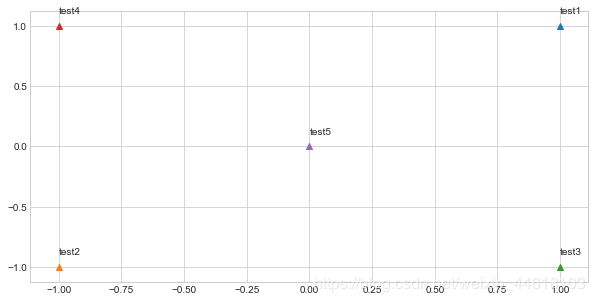
感觉我做的图比他给的样例好看那么一丁点。
Question 1.5: Co-Occurrence Plot Analysis [written] (3 points)
直接根据他提供的代码进行作图就可以了:
# -----------------------------
# Run This Cell to Produce Your Plot
# ------------------------------
reuters_corpus = read_corpus()
M_co_occurrence, word2Ind_co_occurrence = compute_co_occurrence_matrix(reuters_corpus)
M_reduced_co_occurrence = reduce_to_k_dim(M_co_occurrence, k=2)
# Rescale (normalize) the rows to make them each of unit-length
M_lengths = np.linalg.norm(M_reduced_co_occurrence, axis=1)
M_normalized = M_reduced_co_occurrence / M_lengths[:, np.newaxis] # broadcasting
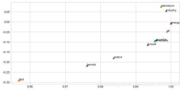
words = ['barrels', 'bpd', 'ecuador', 'energy', 'industry', 'kuwait', 'oil', 'output', 'petroleum', 'venezuela']
plot_embeddings(M_normalized, word2Ind_co_occurrence, words)所作的图如下:
同时老师也提出了几个问题:
Q:
- What clusters together in 2-dimensional embedding space?
- What doesn’t cluster together that you might think should have?
Remark: Note: “bpd” stands for “barrels per day” and is a commonly used abbreviation in crude oil topic articles.
A:
- 可以看到 “petroleum”,“industry” 很相近,“kuwait”,“ecuador”,“venezuela” 这三个词很相近。
- 我认为 “bpd” 应该会与上述词较为接近,因为他们描述的是同样的东西。
-------------------------- 第一部分结束了 -----------------------------
Part 2: Prediction-Based Word Vectors (15 points)
这部分数据集的下载最好事先装好 ,不然非常容易下载失败。
Reducing dimensionality of Word Embeddings
这题是一个比较,比较我们之前写的:利用矩阵 SVD 将其邻接矩阵进行降秩的结果 与 GloVe embeddings 本身数据集中的坐标。
因为邻接矩阵是一个非常稀疏的矩阵,而且数据量极大,这里出题者很好心让我们只用 10000 个单词来进行构造。
Question 2.1: GloVe Plot Analysis [written] (4 points)
这里让我们比较用 co-occurrence 矩阵和用 GloVe embeddings 这个数据里,点的坐标是否有不同。
比较的还是对之前那 10 个单词,运行如下代码:
words = ['barrels', 'bpd', 'ecuador', 'energy', 'industry', 'kuwait', 'oil', 'output', 'petroleum', 'venezuela']
plot_embeddings(M_reduced_normalized, word2Ind, words)
得到的结果如下:

接下来回答作者的问题:
Q:
- What clusters together in 2-dimensional embedding space?
- What doesn’t cluster together that you might think should have?
- How is the plot different from the one generated earlier from the co-occurrence matrix?
- What is a possible reason for causing the difference?
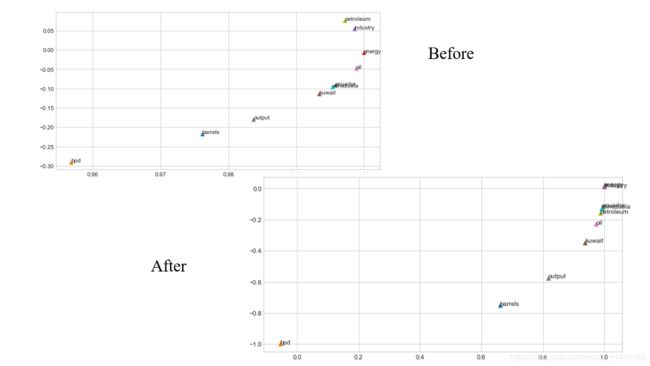
之前的图还得用到,这里把两张图合并一下放一下做对比:
A:
- 可以看到右上角那一堆都聚集在一起了
- 仍然,bpd 这个单词还是离那些单词很远。
- 这张图与之前的不同,之前那张图很明显可以看到有一个右上角往左回拉的一个趋势;新的图却是一个类似凸函数的形状。
- 两幅图的不同,可能来自这部正则化:
M_reduced_normalized = M_reduced / M_lengths[:, np.newaxis] # broadcasting
确实我不太清楚这个引入的数据集中,这些单词的坐标是怎么来的,只能够通过代码入手。如果没有这部正则化,这张图长这样:

这也只是我的个人推测,如果有不同意见,可以评论讨论,共同商讨一下。
Question 2.2: Words with Multiple Meanings (2 points) [code + written]
这题让我们统计一词多义的情况。两个单词之间词义的相似度是由两个向量之间的内积决定的。(因为之前所有单词的坐标到原点的距离都被正则化为 1 1 1 ,因此它们之间的内积就是他们之间夹角 α \alpha α 的 cos α \cos \alpha cosα 值)在这里的处理思路与聚类分析中对距离、相似度的定义是类似的。
这里提示我们使用一个已有的函数:wv_from_bin.most_similar(word) 来完成。这个函数的实现机制是:对所有单词进行求内积,并取内积最大的 10 10 10 个单词返回给你。
这题的思路如下:
首先我引入一个概念:组内离差(这在判断马尔科夫链收敛性中也有使用到)。首先有一个集合(相似集):记录这个单词通过这个 wv_from_bin.most_similar(word) 函数返回的列表。在这个列表中,两两取内积,取其内积最小值,称之为组内离差。
因此,组内离差最小的集合就说明这个单词 与 两个意思相差很远的单词 之间相似度高,也就说明更有可能是一词多义的解。
代码实现如下:
def MultiMeaningWord(M_reduced_normalized, word2Ind):
    wordlst = []
    MultiMeans = ""
    n = len(M_reduced_normalized[0])
    MinVariance = 100
    for word in word2Ind.keys():
        lst = wv_from_bin.most_similar(word)
        cur = 100
        for i in range(10):
            try:
                xy_cur = M_reduced_normalized[word2Ind[lst[i][0]]]
            except KeyError:
                continue
            for j in range(i, 10):
                temp = 0
                try:
                    xy_nxt = M_reduced_normalized[word2Ind[lst[j][0]]]
                except KeyError:
                    continue
                for k in range(n):
                    temp = temp + xy_cur[k] * xy_nxt[k]
                cur = min(cur, temp)
        if cur < MinVariance:
            wordlst = lst
            MinVariance = cur
            MultiMeans = word
    return MultiMeans, wordlst, MinVariance
结果如下:
>>> ('raisonné',
	[('raisonne', 0.6827203035354614),
	('catalogue', 0.6217593550682068),
  	('köchel', 0.5784828662872314),
  	('dictionnaire', 0.5532978773117065),
  	('recueil', 0.538439154624939),
  	('traité', 0.5328050851821899),
  	('hesiodic', 0.5189188718795776),
  	('études', 0.5103318691253662),
  	('etudes', 0.4762265682220459),
  	('encyclopédie', 0.4728423058986664)],
 	-0.9605955556035042)
组间离差为 − 0.96 -0.96 −0.96 是一个相当小的值。然后我们再看这个单词的意思:
raisonné 经过推理的,建立在推理基础上的;思考过的
貌似与剩下的词的意思关系都不是很大,这里存疑,希望见者能够解答一下。
经常会产生这样一个结果:这个词的好几个意思都是相近的,因为意思相近的单词聚类了,他们之间的内积接近于 1 1 1 因此直接取出意思最相近的 10 10 10 个单词很容易造成全部是同义词的情况。
Question 2.3: Synonyms & Antonyms (2 points) [code + written]
这题的主要目的是求同义词和反义词。
具体思路为:
- 选取一个单词,找到与它内积最大的,这个单词就是其近义词;
- 找到与它内积较小的,这个单词就是其反义词。(当然也存在用在语境相同的反义词,这点不是很好判断)
python 实现如下:
def Synonyms_Antonyms(word2Ind, w1):
    words = word2Ind.keys()
    far = ""
    furtherness = 100
    for word in words:
        if word == w1:
            continue
        temp = wv_from_bin.distance(w1, word)
        if furtherness > temp:
            furtherness, far = temp, word
            continue
    return wv_from_bin.most_similar(w1)[0], (far, furtherness)
找符合的单词比较麻烦,最终找到单词:“satisfying” ,执行结果如下:
Res = Synonyms_Antonyms(word2Ind, w1 = 'satisfying')
>>> ([('enjoyable', 0.6154831051826477), ('unsatisfying', 0.4698140621185303))
因此:“satisfying” 的近义词是 “enjoyable” ,反义词是 “unsatisfying” 符合我们的认知。
Solving Analogies with Word Vectors
这一块内容讲的是:通过单词向量来解决问题。这里首先介绍了一个函数:
wv_from_bin.most_similar(positive=['woman', 'king'], negative=['man'])
>>> [('queen', 0.6978678703308105),
	 ('princess', 0.6081745028495789),
	 ('monarch', 0.5889754891395569),
	 ('throne', 0.5775108933448792),
	 ('prince', 0.5750998258590698),
	 ('elizabeth', 0.5463595986366272),
	 ('daughter', 0.5399125814437866),
	 ('kingdom', 0.5318052172660828),
	 ('mother', 0.5168544054031372),
	 ('crown', 0.5164473056793213)]
这里返回的是离 positive 中最近,且离 negative 最远的单词。
Question 2.4: Finding Analogies [code + written] (2 Points)
这题让我们实现一个正确的聚类:
pprint.pprint(wv_from_bin.most_similar(positive=['satisfying', 'exciting'], negative=['unsatisfying']))
>>> [('interesting', 0.6445490121841431),
	 ('really', 0.6026532649993896),
	 ('very', 0.6022480726242065),
	 ('excited', 0.596916675567627),
	 ('wonderful', 0.5959773063659668),
	 ('quite', 0.5956001281738281),
	 ('truly', 0.5935688018798828),
	 ('definitely', 0.5903993248939514),
	 ('entertaining', 0.5786590576171875),
	 ('fun', 0.56939697265625)]
Question 2.5: Incorrect Analogy [code + written] (1 point)
这题是让我们输出一个错误的聚类,实际上挺难找的。如果positive 中存在反义词,那就会导致这个聚类不精确。
pprint.pprint(wv_from_bin.most_similar(positive=['output', 'input'], negative=['energy']))
>>>	[('outputs', 0.6508897542953491),
	 ('inputs', 0.6220414638519287),
	 ('voltage', 0.4847225546836853),
	 ('waveform', 0.4809161126613617),
	 ('audio', 0.46772128343582153),
	 ('amplifier', 0.46416085958480835),
	 ('corresponding', 0.45216110348701477),
	 ('impedance', 0.4518190026283264),
	 ('non-inverting', 0.4489710330963135),
	 ('sequential', 0.4211637079715729)]
Question 2.6: Guided Analysis of Bias in Word Vectors [written] (1 point)
这一节是讲偏差分析的。
pprint.pprint(wv_from_bin.most_similar(positive=['woman', 'worker'], negative=['man']))
print()
pprint.pprint(wv_from_bin.most_similar(positive=['man', 'worker'], negative=['woman']))
输出结果为:
>>> [('employee', 0.6375863552093506),
	 ('workers', 0.6068919897079468),
	 ('nurse', 0.5837947130203247),
	 ('pregnant', 0.5363885760307312),
	 ('mother', 0.5321309566497803),
	 ('employer', 0.5127025842666626),
	 ('teacher', 0.5099577307701111),
	 ('child', 0.5096741914749146),
	 ('homemaker', 0.5019455552101135),
	 ('nurses', 0.4970571994781494)]

	[('workers', 0.611325740814209),
	 ('employee', 0.5983108878135681),
	 ('working', 0.5615329742431641),
	 ('laborer', 0.5442320108413696),
	 ('unemployed', 0.5368517637252808),
	 ('job', 0.5278826951980591),
	 ('work', 0.5223963260650635),
	 ('mechanic', 0.5088937282562256),
	 ('worked', 0.5054520964622498),
	 ('factory', 0.4940453767776489)]
这里输出的是:
- 离男性最远的女性的职业;
- 离女性最远的男性的职业。
之前看到一篇报道说机器学习是有偏见的,没错,机器学习的结果取决于你的训练集。机器学习产生的偏见实际上就是人类自己本身的偏见。
Question 2.7: Independent Analysis of Bias in Word Vectors [code + written] (1 point)
我们需要寻找更多的偏见,一直说女司机,男司机;我们就来看看两个性别之间对驾驶是否存在偏见:
pprint.pprint(wv_from_bin.most_similar(positive=['woman', 'car'], negative=['man']))
print()
pprint.pprint(wv_from_bin.most_similar(positive=['man', 'car'], negative=['woman']))
>>> [('vehicle', 0.6337087750434875),
	 ('cars', 0.6253966689109802),
	 ('driver', 0.6123777031898499),
	 ('truck', 0.5899932384490967),
	 ('minivan', 0.5488290190696716),
	 ('driving', 0.5473644733428955),
	 ('mercedes', 0.5350144505500793),
	 ('parked', 0.5255646109580994),
	 ('vehicles', 0.521051287651062),
	 ('automobile', 0.5183522701263428)]

	[('cars', 0.7136538624763489),
	 ('vehicle', 0.6922875642776489),
	 ('truck', 0.6608046293258667),
	 ('driver', 0.6462159752845764),
	 ('driving', 0.6076016426086426),
	 ('vehicles', 0.5946481227874756),
	 ('motorcycle', 0.5647350549697876),
	 ('drivers', 0.5344247221946716),
	 ('racing', 0.5336049795150757),
	 ('parked', 0.5304452180862427)]
从中可以看到:
- 数值方面,女性是低于男性的。
- 从车辆类型来说,女性偏向 “minivan”,“automobile” 这种车型、男性偏向 “racing”,“motorcycle”
Question 2.8: Thinking About Bias [written] (2 points)
之前也稍微提到了一点偏见是怎么来的,这里稍微总结一下:
- 训练集的偏见。 机器学习产生的结果取决于你的训练集。机器学习产生的偏见实际上就是人类写的文章中带有的偏见。如果文章中经常将 racing 和 man 一起出现,那它们之间的距离会非常近,而到 woman 这个单词就会很远。
- 数据量的不足。 因为我们只引入了10000个词汇量,如果数据量更大一点,说不定能够消除偏见。
- 由于算法设计的原因而导致的偏见。可能有些词的出现拉远了某两个词之间的距离。