Python作业-Jupyter-数据集分析
目标:学习使用Jupyter NoteBook 以及python库中的数据分析函数
exercise链接:
https://nbviewer.jupyter.org/github/schmit/cme193-ipython-notebooks-lecture/blob/master/Exercises.ipynb
题目要求:
1.
Part 1
For each of the four datasets...
- Compute the mean and variance of both x and y
- Compute the correlation coefficient between x and y
- Compute the linear regression line: y=β0+β1x+ϵy=β0+β1x+ϵ (hint: use statsmodels and look at the Statsmodels notebook)
Python代码实现:
%matplotlib inline

import random

import numpy as np
import scipy as sp
import pandas as pd
import matplotlib.pyplot as plt
import seaborn as sns

import statsmodels.api as sm
import statsmodels.formula.api as smf

sns.set_context("talk")

anascombe = pd.read_csv('C:/Users/Administrator/Desktop/data/anscombe.csv')
anascombe.head()

print('The mean of x and y:')
print(anascombe.groupby(['dataset'])[['x', 'y']].mean())

print('\nThe varience of x and y:')
print(anascombe.groupby(['dataset'])[['x', 'y']].var())

print('\nThe correlation coefficient between x and y:')
print(anascombe.groupby(['dataset'])[['x', 'y']].corr());

#hint: use statsmodels and look at the Statsmodels notebook
datasets = ['I', 'II', 'III', 'IV']
for dataset in datasets:
    lin_model = smf.ols('y ~ x', anascombe[anascombe['dataset'] == dataset]).fit()
    print(lin_model.summary())
结果如下:
The mean of x and y:
           x         y
dataset
I        9.0  7.500909
II       9.0  7.500909
III      9.0  7.500000
IV       9.0  7.500909

The varience of x and y:
            x         y
dataset
I        11.0  4.127269
II       11.0  4.127629
III      11.0  4.122620
IV       11.0  4.123249

The correlation coefficient between x and y:
                  x         y
dataset
I       x  1.000000  0.816421
        y  0.816421  1.000000
II      x  1.000000  0.816237
        y  0.816237  1.000000
III     x  1.000000  0.816287
        y  0.816287  1.000000
IV      x  1.000000  0.816521
        y  0.816521  1.000000
                            OLS Regression Results
==============================================================================
Dep. Variable:                      y   R-squared:                       0.667
Model:                            OLS   Adj. R-squared:                  0.629
Method:                 Least Squares   F-statistic:                     17.99
Date:                Mon, 11 Jun 2018   Prob (F-statistic):            0.00217
Time:                        00:06:58   Log-Likelihood:                -16.841
No. Observations:                  11   AIC:                             37.68
Df Residuals:                       9   BIC:                             38.48
Df Model:                           1
Covariance Type:            nonrobust
==============================================================================
                 coef    std err          t      P>|t|      [0.025      0.975]
------------------------------------------------------------------------------
Intercept      3.0001      1.125      2.667      0.026       0.456       5.544
x              0.5001      0.118      4.241      0.002       0.233       0.767
==============================================================================
Omnibus:                        0.082   Durbin-Watson:                   3.212
Prob(Omnibus):                  0.960   Jarque-Bera (JB):                0.289
Skew:                          -0.122   Prob(JB):                        0.865
Kurtosis:                       2.244   Cond. No.                         29.1
==============================================================================

Warnings:
[1] Standard Errors assume that the covariance matrix of the errors is correctly specified.
                            OLS Regression Results
==============================================================================
Dep. Variable:                      y   R-squared:                       0.666
Model:                            OLS   Adj. R-squared:                  0.629
Method:                 Least Squares   F-statistic:                     17.97
Date:                Mon, 11 Jun 2018   Prob (F-statistic):            0.00218
Time:                        00:06:58   Log-Likelihood:                -16.846
No. Observations:                  11   AIC:                             37.69
Df Residuals:                       9   BIC:                             38.49
Df Model:                           1
Covariance Type:            nonrobust
==============================================================================
                 coef    std err          t      P>|t|      [0.025      0.975]
------------------------------------------------------------------------------
Intercept      3.0009      1.125      2.667      0.026       0.455       5.547
x              0.5000      0.118      4.239      0.002       0.233       0.767
==============================================================================
Omnibus:                        1.594   Durbin-Watson:                   2.188
Prob(Omnibus):                  0.451   Jarque-Bera (JB):                1.108
Skew:                          -0.567   Prob(JB):                        0.575
Kurtosis:                       1.936   Cond. No.                         29.1
==============================================================================

Warnings:
[1] Standard Errors assume that the covariance matrix of the errors is correctly specified.
                            OLS Regression Results
==============================================================================
Dep. Variable:                      y   R-squared:                       0.666
Model:                            OLS   Adj. R-squared:                  0.629
Method:                 Least Squares   F-statistic:                     17.97
Date:                Mon, 11 Jun 2018   Prob (F-statistic):            0.00218
Time:                        00:06:58   Log-Likelihood:                -16.838
No. Observations:                  11   AIC:                             37.68
Df Residuals:                       9   BIC:                             38.47
Df Model:                           1
Covariance Type:            nonrobust
==============================================================================
                 coef    std err          t      P>|t|      [0.025      0.975]
------------------------------------------------------------------------------
Intercept      3.0025      1.124      2.670      0.026       0.459       5.546
x              0.4997      0.118      4.239      0.002       0.233       0.766
==============================================================================
Omnibus:                       19.540   Durbin-Watson:                   2.144
Prob(Omnibus):                  0.000   Jarque-Bera (JB):               13.478
Skew:                           2.041   Prob(JB):                      0.00118
Kurtosis:                       6.571   Cond. No.                         29.1
==============================================================================

Warnings:
[1] Standard Errors assume that the covariance matrix of the errors is correctly specified.
                            OLS Regression Results
==============================================================================
Dep. Variable:                      y   R-squared:                       0.667
Model:                            OLS   Adj. R-squared:                  0.630
Method:                 Least Squares   F-statistic:                     18.00
Date:                Mon, 11 Jun 2018   Prob (F-statistic):            0.00216
Time:                        00:06:58   Log-Likelihood:                -16.833
No. Observations:                  11   AIC:                             37.67
Df Residuals:                       9   BIC:                             38.46
Df Model:                           1
Covariance Type:            nonrobust
==============================================================================
                 coef    std err          t      P>|t|      [0.025      0.975]
------------------------------------------------------------------------------
Intercept      3.0017      1.124      2.671      0.026       0.459       5.544
x              0.4999      0.118      4.243      0.002       0.233       0.766
==============================================================================
Omnibus:                        0.555   Durbin-Watson:                   1.662
Prob(Omnibus):                  0.758   Jarque-Bera (JB):                0.524
Skew:                           0.010   Prob(JB):                        0.769
Kurtosis:                       1.931   Cond. No.                         29.1
==============================================================================
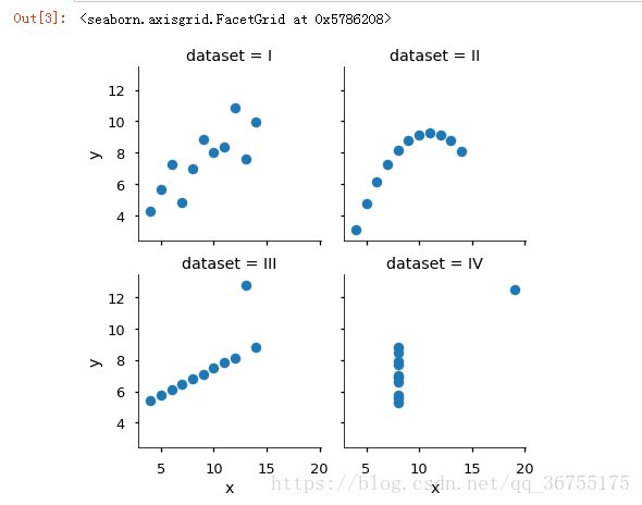
2.
Part 2
Using Seaborn, visualize all four datasets.
hint: use sns.FacetGrid combined with plt.scatter
Python代码:
(参照statsmodels.ipython)
graph= sns.FacetGrid(anascombe, col='dataset',col_wrap=2)
graph.map(plt.scatter, 'x', 'y')
结果如下: