使用贝叶斯方法分类中文垃圾邮件

这里的中文垃圾邮件数据集内含100条正常邮件和50条垃圾邮件，其实，这做为训练数据，是远远不够的。不过，可以先大致看一下中文垃圾邮件处理的过程。

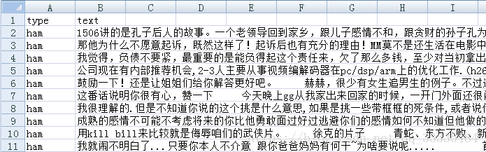
给大家看一下数据集的基本结构，大概是这个样子的：

话不多说，上代码.

导入各种包：

%pylab inline
import matplotlib.pyplot as plt
import pandas as pd
import string
import codecs
import os
import jieba
from sklearn.feature_extraction.text import CountVectorizer
from wordcloud import WordCloud
from sklearn import naive_bayes as bayes
from sklearn.model_selection import train_test_split

打开文件：

#open file
file_path = "C:\\Users\\lenovo\\Documents\\tfstudy"
emailframe = pd.read_excel(os.path.join(file_path, "chinesespam.xlsx"), 0)

检查数据：

#inspect data
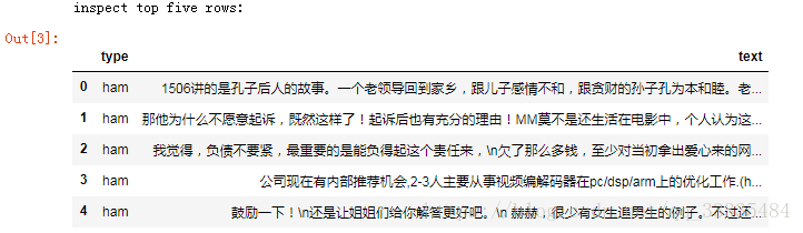
print("inspect top five rows:")
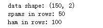
emailframe.head(5)

print("data shape:", emailframe.shape)
print("spams in rows:", emailframe.loc[emailframe['type'] == "spam"].shape[0])
print("ham in rows:", emailframe.loc[emailframe['type'] == "ham"].shape[0])

运行后得到：

可以观察到其中，垃圾邮件50条，非垃圾邮件100条。

载入停止词stopwords：

#load stopwords
stopwords = codecs.open(os.path.join(file_path, 'stopwords.txt'), 'r', 'UTF8').read().split('\r\n')

 

jieba分词，过滤停止词，空字符串，标点等：

#cut words and process text
processed_texts = []
for text in emailframe["text"]:
    words = []
    seg_list = jieba.cut(text)
    for seg in seg_list:
        if (seg.isalpha()) & (seg not in stopwords):
            words.append(seg)
    sentence = " ".join(words)
    processed_texts.append(sentence)
emailframe["text"] = processed_texts

查看过滤后的结果：

#inspect processed text
emailframe.head(3)

 

运行后可以看到：

 

将切词后的数据使用词云展示，观察其中规律：

#word cloud
def showWordCloud(text):
    wc = WordCloud(
    background_color="white",
    max_words=200,
    font_path="C:\\Windows\\Fonts\\STFANGSO.ttf",
    min_font_size=15,
    max_font_size=50, 
    width=400 
    )
    wordcloud = wc.generate(text)
    plt.imshow(wordcloud, interpolation="bilinear")
    plt.axis("off")

#all words cloud
print("all words cloud:")
showWordCloud(" ".join(emailframe["text"]))

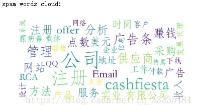
#spam words cloud
print("spam words cloud:")
spamtext = " ".join(emailframe[emailframe["type"] == "spam"]["text"])
showWordCloud(spamtext)

#ham words cloud
print("ham words cloud:")
spamtext = " ".join(emailframe[emailframe["type"] == "ham"]["text"])
showWordCloud(spamtext)

运行后可以观察到， 全部词语组成的词云：

垃圾邮件词语组成的词云：

非垃圾邮件词语组成的词云：

可以观察到，垃圾邮件与非垃圾邮件在词语的组成上，是有区别的。

将数据转变为稀疏矩阵，以便后续的分析：

#transform text to sparse matrix
def transformTextToSparseMatrix(texts):
    vectorizer = CountVectorizer(binary=False)
    vectorizer.fit(texts)

    #inspect vocabulary
    vocabulary = vectorizer.vocabulary_
    print("There are ", len(vocabulary), " word features")
    
    vector = vectorizer.transform(texts)
    result = pd.DataFrame(vector.toarray())
    
    keys = []
    values = []
    for key,value in vectorizer.vocabulary_.items():
        keys.append(key)
        values.append(value)
    df = pd.DataFrame(data = {"key" : keys, "value" : values})
    colnames = df.sort_values("value")["key"].values
    result.columns = colnames
    return result

textmatrix = transformTextToSparseMatrix(emailframe["text"])
textmatrix.head(3)

运行后可以看到：

数据集中一共有5982个不同的单词，即有5982个不同的特征。维数太多，于是接下来剔除一些频繁词汇，降低维度

#pop freq words
features = pd.DataFrame(textmatrix.apply(sum, axis=0))
extractedfeatures = [features.index[i] for i in range(features.shape[0]) if features.iloc[i, 0] > 5]
textmatrix = textmatrix[extractedfeatures]
print("There are ", textmatrix.shape[1], " word features")

剔除了其中词频 > 5 的单词，运行后

只剩下544个单词，然后切分训练集和测试集

#traindate & testdata
train, test, trainlabel, testlabel = train_test_split(textmatrix, emailframe["type"], test_size = 0.2)

使用朴素贝叶斯训练模型：

#train model
clf = bayes.BernoulliNB(alpha=1, binarize=True)
model = clf.fit(train, trainlabel)

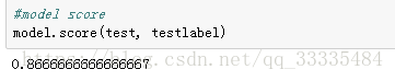
最后模型评分：

#model score
model.score(test, testlabel)

可以观察到评分：

代码githup下载地址：

https://github.com/freeingfree/test