【机器学习实用指南】加州房价中位数预测
加州房价预测
# 同时支持python2和python3
from __future__ import division,print_function,unicode_literals

# 常用库
import numpy as np
import os

# 使这个notebook的输出一直是不变的
np.random.seed(42)

# 用于画图的库
import matplotlib as mpl
import matplotlib.pyplot as plt
mpl.rc('axes', labelsize=14)
mpl.rc('xtick', labelsize=12)
mpl.rc('ytick', labelsize=12)
%matplotlib inline

# 用于保存图片
PROJECT_ROOT_DIR = "."
CHAPTER_ID = "end_to_end_project"
IMAGES_PATH = os.path.join(PROJECT_ROOT_DIR, "images", CHAPTER_ID)

def save_fig(fig_id, tight_layout=True, fig_extension="png", resolution=300):
    path = os.path.join(IMAGES_PATH, fig_id + "." + fig_extension)
    print("Saving figure", fig_id)
    if tight_layout:
        plt.tight_layout()
    plt.savefig(path, format=fig_extension, dpi=resolution)

# 去除代码警告
import warnings
warnings.filterwarnings(action="ignore", message="^internal gelsd")
1.获取数据
import os
import tarfile #https://www.jianshu.com/p/5609d67d8ab2
from six.moves import urllib  #https://www.bbsmax.com/A/WpdKAmkZJV/

DOWNLOAD_ROOT = "https://raw.githubusercontent.com/ageron/handson-ml/master/"
HOUSING_PATH = os.path.join("datasets", "housing")
HOUSING_URL = DOWNLOAD_ROOT + "datasets/housing/housing.tgz"

def fetch_housing_data(housing_url=HOUSING_URL, housing_path=HOUSING_PATH):
    os.makedirs(housing_path, exist_ok=True)
    tgz_path = os.path.join(housing_path, "housing.tgz")
    urllib.request.urlretrieve(housing_url, tgz_path)
    housing_tgz = tarfile.open(tgz_path)
    housing_tgz.extractall(path=housing_path)
    housing_tgz.close()
# fetch_housing_data()
# 读取数据
import pandas as pd

def load_housing_data(housing_path=HOUSING_PATH):
    csv_path = os.path.join(housing_path, "housing.csv")
    return pd.read_csv(csv_path)
每一行都表示一个街区。共有 10 个属性(截图中可以看到 6 个):经度、维度、房屋年龄中 位数、总房间数、总卧室数、人口数、家庭数、收入中位数、房屋价值中位数、离大海距 离。
housing = load_housing_data()
housing.head()
| longitude | latitude | housing_median_age | total_rooms | total_bedrooms | population | households | median_income | median_house_value | ocean_proximity | |
|---|---|---|---|---|---|---|---|---|---|---|
| 0 | -122.23 | 37.88 | 41.0 | 880.0 | 129.0 | 322.0 | 126.0 | 8.3252 | 452600.0 | NEAR BAY |
| 1 | -122.22 | 37.86 | 21.0 | 7099.0 | 1106.0 | 2401.0 | 1138.0 | 8.3014 | 358500.0 | NEAR BAY |
| 2 | -122.24 | 37.85 | 52.0 | 1467.0 | 190.0 | 496.0 | 177.0 | 7.2574 | 352100.0 | NEAR BAY |
| 3 | -122.25 | 37.85 | 52.0 | 1274.0 | 235.0 | 558.0 | 219.0 | 5.6431 | 341300.0 | NEAR BAY |
| 4 | -122.25 | 37.85 | 52.0 | 1627.0 | 280.0 | 565.0 | 259.0 | 3.8462 | 342200.0 | NEAR BAY |
info() 方法可以快速查看数据的描述,特别是总行数、每个属性的类型和非空值的数量。
housing.info()
RangeIndex: 20640 entries, 0 to 20639
Data columns (total 10 columns):
 #   Column              Non-Null Count  Dtype
---  ------              --------------  -----
 0   longitude           20640 non-null  float64
 1   latitude            20640 non-null  float64
 2   housing_median_age  20640 non-null  float64
 3   total_rooms         20640 non-null  float64
 4   total_bedrooms      20433 non-null  float64
 5   population          20640 non-null  float64
 6   households          20640 non-null  float64
 7   median_income       20640 non-null  float64
 8   median_house_value  20640 non-null  float64
 9   ocean_proximity     20640 non-null  object
dtypes: float64(9), object(1)
memory usage: 1.6+ MB
数据集中共有 20640 个实例,按照机器学习的标准这个数据量很小,但是非常适合入门。我 们注意到总房间数只有 20433 个非空值,这意味着有 207 个街区缺少这个值。我们将在后面 对它进行处理。
所有的属性都是数值的,除了离大海距离这项。它的类型是对象,因此可以包含任意 Python 对象,但是因为该项是从 CSV 文件加载的,所以必然是文本类型
housing["ocean_proximity"].value_counts()
<1H OCEAN     9136
INLAND        6551
NEAR OCEAN    2658
NEAR BAY      2290
ISLAND           5
Name: ocean_proximity, dtype: int64
housing.describe()
| longitude | latitude | housing_median_age | total_rooms | total_bedrooms | population | households | median_income | median_house_value | |
|---|---|---|---|---|---|---|---|---|---|
| count | 20640.000000 | 20640.000000 | 20640.000000 | 20640.000000 | 20433.000000 | 20640.000000 | 20640.000000 | 20640.000000 | 20640.000000 |
| mean | -119.569704 | 35.631861 | 28.639486 | 2635.763081 | 537.870553 | 1425.476744 | 499.539680 | 3.870671 | 206855.816909 |
| std | 2.003532 | 2.135952 | 12.585558 | 2181.615252 | 421.385070 | 1132.462122 | 382.329753 | 1.899822 | 115395.615874 |
| min | -124.350000 | 32.540000 | 1.000000 | 2.000000 | 1.000000 | 3.000000 | 1.000000 | 0.499900 | 14999.000000 |
| 25% | -121.800000 | 33.930000 | 18.000000 | 1447.750000 | 296.000000 | 787.000000 | 280.000000 | 2.563400 | 119600.000000 |
| 50% | -118.490000 | 34.260000 | 29.000000 | 2127.000000 | 435.000000 | 1166.000000 | 409.000000 | 3.534800 | 179700.000000 |
| 75% | -118.010000 | 37.710000 | 37.000000 | 3148.000000 | 647.000000 | 1725.000000 | 605.000000 | 4.743250 | 264725.000000 |
| max | -114.310000 | 41.950000 | 52.000000 | 39320.000000 | 6445.000000 | 35682.000000 | 6082.000000 | 15.000100 | 500001.000000 |
count 、 mean 、 min 和 max 几行的意思很明显了。注意,空值被忽略了(所以,卧室总数 是 20433 而不是 20640)。 std 是标准差(揭示数值的分散度)。25%、50%、75% 展示了 对应的分位数:每个分位数指明小于这个值,且指定分组的百分比。例如,25% 的街区的房 屋年龄中位数小于 18,而 50% 的小于 29,75% 的小于 37。这些值通常称为第 25 个百分位 数(或第一个四分位数),中位数,第 75 个百分位数(第三个四分位数)。
# 画出数据分布直方图
housing.hist()

housing.hist(bins=50, figsize=(20,15))
save_fig("attribute_histogram_plots")
plt.show()
Saving figure attribute_histogram_plots
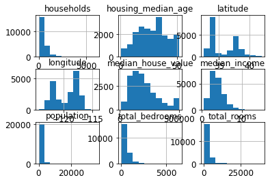
房屋年龄中位数和房屋价值中位数也被设了上限。后者可能是个严重的问题,因为它是 你的目标属性(你的标签)。你的机器学习算法可能学习到价格不会超出这个界限。你 需要与下游团队核实,这是否会成为问题。如果他们告诉你他们需要明确的预测值,即 使超过 500000 美元,你则有两个选项:
i. 对于设了上限的标签,重新收集合适的标签;
ii. 将这些街区从训练集移除(也从测试集移除,因为若房价超出 500000 美元,你的系 统就会被差评)。
describe() 方法展示了数值属性的概括
# 数据集拆分
from sklearn.model_selection import train_test_split

train_set, test_set = train_test_split(housing, test_size=0.2, random_state=42)
test_set.head()
| longitude | latitude | housing_median_age | total_rooms | total_bedrooms | population | households | median_income | median_house_value | ocean_proximity | |
|---|---|---|---|---|---|---|---|---|---|---|
| 20046 | -119.01 | 36.06 | 25.0 | 1505.0 | NaN | 1392.0 | 359.0 | 1.6812 | 47700.0 | INLAND |
| 3024 | -119.46 | 35.14 | 30.0 | 2943.0 | NaN | 1565.0 | 584.0 | 2.5313 | 45800.0 | INLAND |
| 15663 | -122.44 | 37.80 | 52.0 | 3830.0 | NaN | 1310.0 | 963.0 | 3.4801 | 500001.0 | NEAR BAY |
| 20484 | -118.72 | 34.28 | 17.0 | 3051.0 | NaN | 1705.0 | 495.0 | 5.7376 | 218600.0 | <1H OCEAN |
| 9814 | -121.93 | 36.62 | 34.0 | 2351.0 | NaN | 1063.0 | 428.0 | 3.7250 | 278000.0 | NEAR OCEAN |
housing["median_income"].hist(bins=30)
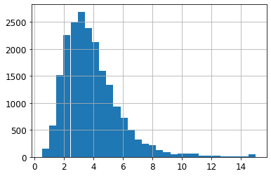
sklearn所提供的方法是随机采样。当数据集很大时(与属性数相比),这通常是可行的,但如果数据集不大时,就会有采样偏差的风险,意思是我们的采样对于整体样本应具有代表性。所以这里可以使用分层采样。
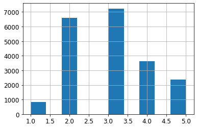
又因为收入中位数被视为一个重要属性,所以对于采样的数据必须包含收入中位数的各个区间,以让数据具有代表性。又根据分布直方图可直收入中位数主要分布在2-5(万美元)。我们将数据进行分层,并保证每个分层足够大,所以我们在这里将收入中位数除以1.5,使数据足够“集中”,从而限制收入分类的数量。
# Divide by 1.5 to limit the number of income categories
housing["income_cat"] = np.ceil(housing["median_income"] / 1.5)
# Label those above 5 as 5
housing["income_cat"].where(housing["income_cat"] < 5, 5.0, inplace=True)
同时也可以使用pandas所提供得函数,如下:
# pd.cut()用于离散区间,并打上标签
#https://blog.csdn.net/qq_35290785/article/details/102622043

# 将大于6的值看作5
housing["income_cat"] = pd.cut(housing["median_income"],
                              bins=[0.,1.5,3.0,4.5,6.,np.inf],
                              labels=[1,2,3,4,5])

## 保证所有数据能够显示,而不是用省略号表示,np.inf表示一个足够大的数
# 打印值的分布

housing["income_cat"].value_counts()
3    7236
2    6581
4    3639
5    2362
1     822
Name: income_cat, dtype: int64
# 输出housing_cat的分布直方图

housing["income_cat"].hist()
根据分类进行分层采样,这里使用sklearn提供的StratifiedShuffleSplit类
from sklearn.model_selection import StratifiedShuffleSplit

split = StratifiedShuffleSplit(n_splits=1, test_size=0.2, random_state=42)
for train_index, test_index in split.split(housing, housing["income_cat"]):
    strat_train_set = housing.loc[train_index]
    strat_test_set = housing.loc[test_index]
strat_test_set["income_cat"].value_counts() / len(strat_test_set) #打印各个分类所占的比例
3    0.350533
2    0.318798
4    0.176357
5    0.114583
1    0.039729
Name: income_cat, dtype: float64
housing["income_cat"].value_counts() / len(housing)
3    0.350581
2    0.318847
4    0.176308
5    0.114438
1    0.039826
Name: income_cat, dtype: float64
# 恢复数据集,在训练集和测试集中删除income_cat属性
for set in (strat_train_set, strat_test_set):
    set.drop(["income_cat"], axis=1, inplace=True)
对比总数据集、分层采样 的测试集、纯随机采样测试集的收入分类比例。
def income_cat_proportions(data):
    return data["income_cat"].value_counts() / len(data)

train_set, test_set = train_test_split(housing, test_size=0.2, random_state=42)

compare_props = pd.DataFrame({
    "Overall": income_cat_proportions(housing),
    "Stratified": income_cat_proportions(strat_test_set),
    "Random": income_cat_proportions(test_set),
}).sort_index()
compare_props["Rand. %error"] = 100 * compare_props["Random"] / compare_props["Overall"] - 100
compare_props["Strat. %error"] = 100 * compare_props["Stratified"] / compare_props["Overall"] - 100
2.数据探索和可视化,发现规律
# copy数据集并对数据集进行探索
housing = strat_train_set.copy()
使用pandas可视化地理信息
#
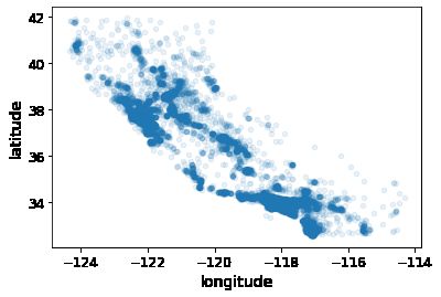
housing.plot(kind="scatter", x="longitude", y="latitude",alpha=0.1)
。每个圈的半径表示街区的人口(选项 s ),颜色代表价格(选 项 c )。我们用预先定义的名为 jet 的颜色图(选项 cmap ),它的范围是从蓝色(低价) 到红色(高价):
housing.plot(kind="scatter", x="longitude", y="latitude", alpha=0.4,
    s=housing["population"]/100, label="population", figsize=(10,7),
    c="median_house_value", cmap=plt.get_cmap("jet"), colorbar=True,
    sharex=False)
plt.legend()
save_fig("housing_prices_scatterplot")
Saving figure housing_prices_scatterplot
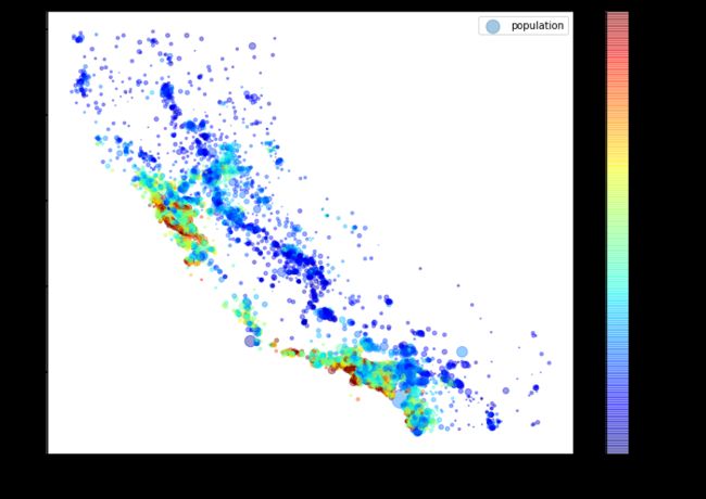
这张图说明房价和位置(比如,靠海)和人口密度联系密切,这点你可能早就知道。可以使 用聚类算法来检测主要的聚集,用一个新的特征值测量聚集中心的距离。尽管北加州海岸区 域的房价不是非常高,但离大海距离属性也可能很有用,所以这不是用一个简单的规则就可 以定义的问题。
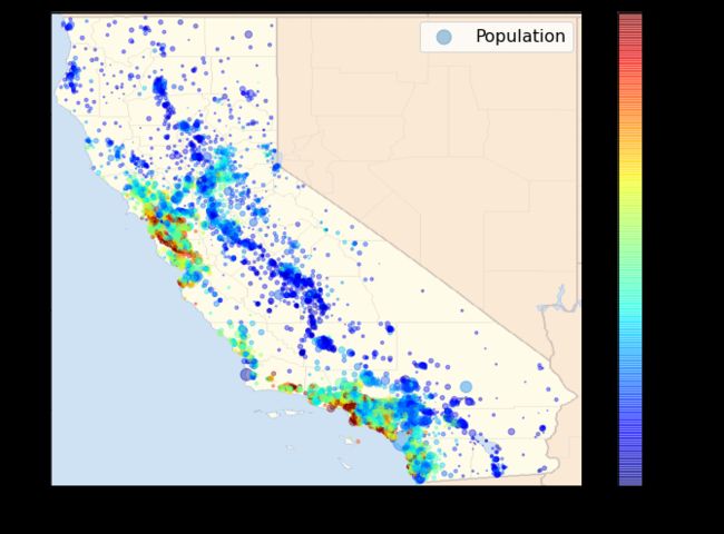
import matplotlib.image as mpimg
california_img=mpimg.imread(PROJECT_ROOT_DIR + '/images/end_to_end_project/california.png')
ax = housing.plot(kind="scatter", x="longitude", y="latitude", figsize=(10,7),
                       s=housing['population']/100, label="Population",
                       c="median_house_value", cmap=plt.get_cmap("jet"),
                       colorbar=False, alpha=0.4,
                      )
plt.imshow(california_img, extent=[-124.55, -113.80, 32.45, 42.05], alpha=0.5,
           cmap=plt.get_cmap("jet"))
plt.ylabel("Latitude", fontsize=14)
plt.xlabel("Longitude", fontsize=14)

prices = housing["median_house_value"]
tick_values = np.linspace(prices.min(), prices.max(), 11)
cbar = plt.colorbar()
cbar.ax.set_yticklabels(["$%dk"%(round(v/1000)) for v in tick_values], fontsize=14)
cbar.set_label('Median House Value', fontsize=16)

plt.legend(fontsize=16)
save_fig("california_housing_prices_plot")
plt.show()
Saving figure california_housing_prices_plot
3.查找关联
因为数据集并不是非常大,你可以很容易地使用 corr() 方法计算出每对属性间的标准相关系 数(standard correlation coefficient,也称作皮尔逊相关系数):
相关系数的范围是 -1 到 1。当接近 1 时,意味强正相关;例如,当收入中位数增加时,房价 中位数也会增加。当相关系数接近 -1 时,意味强负相关;你可以看到,纬度和房价中位数有 轻微的负相关性(即,越往北,房价越可能降低)。最后,相关系数接近 0,意味没有线性相 关性。
corr_matrix = housing.corr()
corr_matrix["median_house_value"].sort_values(ascending=False) #关联性按从大到小排序
median_house_value    1.000000
median_income         0.687160
total_rooms           0.135097
housing_median_age    0.114110
households            0.064506
total_bedrooms        0.047689
population           -0.026920
longitude            -0.047432
latitude             -0.142724
Name: median_house_value, dtype: float64
警告:相关系数只测量线性关系(如果 x 上升, y 则上升或下降)。相关系数可能会完 全忽略非线性关系(例如,如果 x 接近 0,则 y 值会变高)。在上面图片的最后一行 中,他们的相关系数都接近于 0,尽管它们的轴并不独立:这些就是非线性关系的例 子。另外,第二行的相关系数等于 1 或 -1;这和斜率没有任何关系。例如,你的身高 (单位是英寸)与身高(单位是英尺或纳米)的相关系数就是 1。
使用pandas的scatter_matrix 函数,它能画出每个数 值属性对每个其它数值属性的图。用于考察属性间的相关系数。
画出散点矩阵
# 从pandas.tools.plotting 导入scatter_matrix
from pandas.plotting import scatter_matrix

attributes = ["median_house_value", "median_income", "total_rooms",
              "housing_median_age"]
scatter_matrix(housing[attributes], figsize=(12, 8))
save_fig("scatter_matrix_plot")
Saving figure scatter_matrix_plot

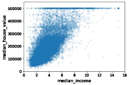
如果 pandas 将每个变量对自己作图,主对角线(左上到右下)都会是直线图。所以 Pandas 展示的是每个属性的柱状图(也可以是其它的,请参考 Pandas 文档)。 最有希望用来预测房价中位数的属性是收入中位数,因此将这张图放大
housing.plot(kind="scatter", x="median_income", y="median_house_value",
             alpha=0.1)
plt.axis([0, 16, 0, 550000])
save_fig("income_vs_house_value_scatterplot")
Saving figure income_vs_house_value_scatterplot
housing.describe()
| longitude | latitude | housing_median_age | total_rooms | total_bedrooms | population | households | median_income | median_house_value | rooms_per_household | bedrooms_per_room | population_per_household | |
|---|---|---|---|---|---|---|---|---|---|---|---|---|
| count | 16512.000000 | 16512.000000 | 16512.000000 | 16512.000000 | 16354.000000 | 16512.000000 | 16512.000000 | 16512.000000 | 16512.000000 | 16512.000000 | 16354.000000 | 16512.000000 |
| mean | -119.575834 | 35.639577 | 28.653101 | 2622.728319 | 534.973890 | 1419.790819 | 497.060380 | 3.875589 | 206990.920724 | 5.440341 | 0.212878 | 3.096437 |
| std | 2.001860 | 2.138058 | 12.574726 | 2138.458419 | 412.699041 | 1115.686241 | 375.720845 | 1.904950 | 115703.014830 | 2.611712 | 0.057379 | 11.584826 |
| min | -124.350000 | 32.540000 | 1.000000 | 6.000000 | 2.000000 | 3.000000 | 2.000000 | 0.499900 | 14999.000000 | 1.130435 | 0.100000 | 0.692308 |
| 25% | -121.800000 | 33.940000 | 18.000000 | 1443.000000 | 295.000000 | 784.000000 | 279.000000 | 2.566775 | 119800.000000 | 4.442040 | 0.175304 | 2.431287 |
| 50% | -118.510000 | 34.260000 | 29.000000 | 2119.500000 | 433.000000 | 1164.000000 | 408.000000 | 3.540900 | 179500.000000 | 5.232284 | 0.203031 | 2.817653 |
| 75% | -118.010000 | 37.720000 | 37.000000 | 3141.000000 | 644.000000 | 1719.250000 | 602.000000 | 4.744475 | 263900.000000 | 6.056361 | 0.239831 | 3.281420 |
| max | -114.310000 | 41.950000 | 52.000000 | 39320.000000 | 6210.000000 | 35682.000000 | 5358.000000 | 15.000100 | 500001.000000 | 141.909091 | 1.000000 | 1243.333333 |
这张图说明了几点。首先,相关性非常高;可以清晰地看到向上的趋势,并且数据点不是非 常分散。第二,我们之前看到的最高价,清晰地呈现为一条位于 500000 美元的水平线。这张 图也呈现了一些不是那么明显的直线:一条位于 450000 美元的直线,一条位于 350000 美元 的直线,一条在 280000 美元的线,和一些更靠下的线。你可能希望去除对应的街区,以防止 算法重复这些巧合。
4. 属性组合实验
**在前面的操作中我们发现了一些数据的巧合,需要 在给算法提供数据之前,将其去除。我们还发现了一些属性间有趣的关联,特别是目标属性。 我们还注意到一些属性具有长尾分布,因此我们可能要将其进行转换(例如,计算其 log 对 数)。当然,不同项目的处理方法各不相同,但大体思路是相似的。
**
给算法准备数据之前,你需要做的最后一件事是尝试多种属性组合。例如,如果你不知道某 个街区有多少户,该街区的总房间数就没什么用。你真正需要的是每户有几个房间。相似 的,总卧室数也不重要:你可能需要将其与房间数进行比较。每户的人口数也是一个有趣的 属性组合。让我们来创建这些新的属性:
housing["rooms_per_household"] = housing["total_rooms"]/housing["households"]
housing["bedrooms_per_room"] = housing["total_bedrooms"]/housing["total_rooms"]
housing["population_per_household"]=housing["population"]/housing["households"]
打印关联矩阵
corr_matrix = housing.corr()
corr_matrix["median_house_value"].sort_values(ascending=False)
median_house_value          1.000000
median_income               0.688075
rooms_per_household         0.151948
total_rooms                 0.134153
housing_median_age          0.105623
households                  0.065843
total_bedrooms              0.049686
population_per_household   -0.023737
population                 -0.024650
longitude                  -0.045967
latitude                   -0.144160
bedrooms_per_room          -0.255880
Name: median_house_value, dtype: float64
与总房间数或卧室数相比,新的 bedrooms_per_room 属性与房价中位数的关联更 强。显然,卧室数/总房间数的比例越低,房价就越高。每户的房间数也比街区的总房间数的 更有信息,很明显,房屋越大,房价就越高。
5.为机器学习算法准备数据
现在来为机器学习算法准备数据。不要手工来做,你需要写一些函数,理由如下:
- 函数可以让你在任何数据集上(比如,你下一次获取的是一个新的数据集)方便地进行 重复数据转换。
- 你能慢慢建立一个转换函数库,可以在未来的项目中复用。
- 在将数据传给算法之前,你可以在实时系统中使用这些函数。
- 这可以让你方便地尝试多种数据转换,查看哪些转换方法结合起来效果最好。
但是,还是先回到干净的训练集(通过再次复制 strat_train_set ),将预测量和标签分开, 因为我们不想对预测量和目标值应用相同的转换(注意 drop() 创建了一份数据的备份,而不 影响 strat_train_set ):
housing = strat_train_set.drop("median_house_value", axis=1) #从训练集中删除标签列
housing_labels = strat_train_set["median_house_value"].copy()
# 打印出不完整的样本行
sample_incomplete_rows = housing[housing.isnull().any(axis=1)].head()
sample_incomplete_rows
| longitude | latitude | housing_median_age | total_rooms | total_bedrooms | population | households | median_income | ocean_proximity | |
|---|---|---|---|---|---|---|---|---|---|
| 4629 | -118.30 | 34.07 | 18.0 | 3759.0 | NaN | 3296.0 | 1462.0 | 2.2708 | <1H OCEAN |
| 6068 | -117.86 | 34.01 | 16.0 | 4632.0 | NaN | 3038.0 | 727.0 | 5.1762 | <1H OCEAN |
| 17923 | -121.97 | 37.35 | 30.0 | 1955.0 | NaN | 999.0 | 386.0 | 4.6328 | <1H OCEAN |
| 13656 | -117.30 | 34.05 | 6.0 | 2155.0 | NaN | 1039.0 | 391.0 | 1.6675 | INLAND |
| 19252 | -122.79 | 38.48 | 7.0 | 6837.0 | NaN | 3468.0 | 1405.0 | 3.1662 | <1H OCEAN |
6. 数据清洗
# 删除在total_bedrooms含有空数据的全部行 方法一
# https://www.jianshu.com/p/89de6c085d22

sample_incomplete_rows.dropna(subset=["total_bedrooms"])
| longitude | latitude | housing_median_age | total_rooms | total_bedrooms | population | households | median_income | ocean_proximity |
|---|
# 删除total_bedrooms属性列 方法二
sample_incomplete_rows.drop("total_bedrooms",axis=1)
| longitude | latitude | housing_median_age | total_rooms | population | households | median_income | ocean_proximity | |
|---|---|---|---|---|---|---|---|---|
| 4629 | -118.30 | 34.07 | 18.0 | 3759.0 | 3296.0 | 1462.0 | 2.2708 | <1H OCEAN |
| 6068 | -117.86 | 34.01 | 16.0 | 4632.0 | 3038.0 | 727.0 | 5.1762 | <1H OCEAN |
| 17923 | -121.97 | 37.35 | 30.0 | 1955.0 | 999.0 | 386.0 | 4.6328 | <1H OCEAN |
| 13656 | -117.30 | 34.05 | 6.0 | 2155.0 | 1039.0 | 391.0 | 1.6675 | INLAND |
| 19252 | -122.79 | 38.48 | 7.0 | 6837.0 | 3468.0 | 1405.0 | 3.1662 | <1H OCEAN |
# 通过fillna填充缺失值
# https://www.jianshu.com/p/79086fa52803

median = housing["total_bedrooms"].median()
sample_incomplete_rows["total_bedrooms"].fillna(median, inplace=True) # option 3
sample_incomplete_rows
使用sklearn的Imputer类处理缺失值
try:
    from sklearn.impute import SimpleImputer # Scikit-Learn 0.20+
except ImportError:
    from sklearn.preprocessing import Imputer as SimpleImputer

imputer = SimpleImputer(strategy="median")
# 因为Imputer只能处理数值属性,所以需要删除文本属性ocean_proximity
housing_num = housing.drop('ocean_proximity', axis=1)
# 或者使用: housing_num = housing.select_dtypes(include=[np.number])
imputer.fit(housing_num)
SimpleImputer(add_indicator=False, copy=True, fill_value=None,
              missing_values=nan, strategy='median', verbose=0)
# 输出每个属性的中位数
imputer.statistics_
array([-118.51  ,   34.26  ,   29.    , 2119.5   ,  433.    , 1164.    ,
        408.    ,    3.5409])
# 检查这是否与手动计算每个属性的中位数相同:
housing_num.median().values
array([-118.51  ,   34.26  ,   29.    , 2119.5   ,  433.    , 1164.    ,
        408.    ,    3.5409])
将缺失值转换为中位数
X = imputer.transform(housing_num)
housing_tr = pd.DataFrame(X, columns=housing_num.columns,
                          index=housing.index)
housing_tr.loc[sample_incomplete_rows.index.values]
| longitude | latitude | housing_median_age | total_rooms | total_bedrooms | population | households | median_income | |
|---|---|---|---|---|---|---|---|---|
| 4629 | -118.30 | 34.07 | 18.0 | 3759.0 | 433.0 | 3296.0 | 1462.0 | 2.2708 |
| 6068 | -117.86 | 34.01 | 16.0 | 4632.0 | 433.0 | 3038.0 | 727.0 | 5.1762 |
| 17923 | -121.97 | 37.35 | 30.0 | 1955.0 | 433.0 | 999.0 | 386.0 | 4.6328 |
| 13656 | -117.30 | 34.05 | 6.0 | 2155.0 | 433.0 | 1039.0 | 391.0 | 1.6675 |
| 19252 | -122.79 | 38.48 | 7.0 | 6837.0 | 433.0 | 3468.0 | 1405.0 | 3.1662 |
imputer.strategy
'median'
# 将数据重新转换为DataFrame
housing_tr = pd.DataFrame(X, columns=housing_num.columns,
                          index=housing_num.index)
housing_tr.head()
| longitude | latitude | housing_median_age | total_rooms | total_bedrooms | population | households | median_income | |
|---|---|---|---|---|---|---|---|---|
| 17606 | -121.89 | 37.29 | 38.0 | 1568.0 | 351.0 | 710.0 | 339.0 | 2.7042 |
| 18632 | -121.93 | 37.05 | 14.0 | 679.0 | 108.0 | 306.0 | 113.0 | 6.4214 |
| 14650 | -117.20 | 32.77 | 31.0 | 1952.0 | 471.0 | 936.0 | 462.0 | 2.8621 |
| 3230 | -119.61 | 36.31 | 25.0 | 1847.0 | 371.0 | 1460.0 | 353.0 | 1.8839 |
| 3555 | -118.59 | 34.23 | 17.0 | 6592.0 | 1525.0 | 4459.0 | 1463.0 | 3.0347 |
Scikit-Learn 设计
Scikit-Learn 设计的 API 设计的非常好。它的主要设计原则是:
一致性:所有对象的接口一致且简单:
估计器(estimator)。任何可以基于数据集对一些参数进行估计的对象都被称 为估计器(比如, imputer 就是个估计器)。估计本身是通过 fit() 方法,只 需要一个数据集作为参数(对于监督学习算法,需要两个数据集;第二个数据 集包含标签)。任何其它用来指导估计过程的参数都被当做超参数(比 如 imputer 的 strategy ),并且超参数要被设置成实例变量(通常通过构造器 参数设置)。
转换器(transformer)。一些估计器(比如 imputer )也可以转换数据集,这 些估计器被称为转换器。API也是相当简单:转换是通过 transform() 方法,被 转换的数据集作为参数。返回的是经过转换的数据集。转换过程依赖学习到的 参数,比如 imputer 的例子。所有的转换都有一个便捷的方 法 fit_transform() ,等同于调用 fit() 再 transform() (但有 时 fit_transform() 经过优化,运行的更快)。
预测器(predictor)。最后,一些估计器可以根据给出的数据集做预测,这些 估计器称为预测器。例如,上一章的 LinearRegression 模型就是一个预测器: 它根据一个国家的人均 GDP 预测生活满意度。预测器有一个 predict() 方法, 可以用新实例的数据集做出相应的预测。预测器还有一个 score() 方法,可以 根据测试集(和相应的标签,如果是监督学习算法的话)对预测进行衡器。
可检验。所有估计器的超参数都可以通过实例的public变量直接访问(比 如, imputer.strategy ),并且所有估计器学习到的参数也可以通过在实例变量名 后加下划线来访问(比如, imputer.statistics_ )。
类不可扩散。数据集被表示成 NumPy 数组或 SciPy 稀疏矩阵,而不是自制的类。 超参数只是普通的 Python 字符串或数字。
可组合。尽可能使用现存的模块。例如,用任意的转换器序列加上一个估计器,就 可以做成一个流水线,后面会看到例子。
合理的默认值。Scikit-Learn 给大多数参数提供了合理的默认值,很容易就能创建一 个系统。
7.处理文本和类别属性
将文字属性 ocean_proximity 转换为数值属性
这里使用sklearn提供的转换器 OrdinalEncoder
提取 ocean_proximity 属性
housing_cat = housing[['ocean_proximity']]
housing_cat.head(10)
| ocean_proximity | |
|---|---|
| 17606 | <1H OCEAN |
| 18632 | <1H OCEAN |
| 14650 | NEAR OCEAN |
| 3230 | INLAND |
| 3555 | <1H OCEAN |
| 19480 | INLAND |
| 8879 | <1H OCEAN |
| 13685 | INLAND |
| 4937 | <1H OCEAN |
| 4861 | <1H OCEAN |
# 导入函数库
try:
    from sklearn.preprocessing import OrdinalEncoder
except ImportError:
    from future_encoders import OrdinalEncoder # Scikit-Learn < 0.20
ordinal_encoder = OrdinalEncoder()
housing_cat_encoded = ordinal_encoder.fit_transform(housing_cat)
housing_cat_encoded[:10]
array([[0.],
       [0.],
       [4.],
       [1.],
       [0.],
       [1.],
       [0.],
       [1.],
       [0.],
       [0.]])
ordinal_encoder.categories_
[array(['<1H OCEAN', 'INLAND', 'ISLAND', 'NEAR BAY', 'NEAR OCEAN'],
       dtype=object)]
这种做法的问题是,ML 算法会认为两个临近的值比两个疏远的值要更相似。显然这样不对 (比如,分类 0 和 4 比 0 和 1 更相似)。这里使用One-hot编码进行处理。
try:
    from sklearn.preprocessing import OrdinalEncoder # just to raise an ImportError if Scikit-Learn < 0.20
    from sklearn.preprocessing import OneHotEncoder
except ImportError:
    from future_encoders import OneHotEncoder # Scikit-Learn < 0.20

cat_encoder = OneHotEncoder()
# cat_encoder = OneHotEncoder(sparse=False) 输出为Numpy数组,而不是系数矩阵
housing_cat_1hot = cat_encoder.fit_transform(housing_cat)
housing_cat_1hot
<16512x5 sparse matrix of type ''
	with 16512 stored elements in Compressed Sparse Row format>
# OneHotEncoder返回一个稀疏矩阵,这里需要将其转换为密集Numpy数组
housing_cat_1hot.toarray()
array([[1., 0., 0., 0., 0.],
       [1., 0., 0., 0., 0.],
       [0., 0., 0., 0., 1.],
       ...,
       [0., 1., 0., 0., 0.],
       [1., 0., 0., 0., 0.],
       [0., 0., 0., 1., 0.]])
cat_encoder.categories_
[array(['<1H OCEAN', 'INLAND', 'ISLAND', 'NEAR BAY', 'NEAR OCEAN'],
       dtype=object)]
8. 创建一个自定义转换器以添加额外的属性
我们需要让自制的转换器与 Scikit-Learn 组件(比如流水线)无 缝衔接工作,因为 Scikit-Learn 是依赖鸭子类型的(而不是继承),你所需要做的是创建一个 类并执行三个方法: fit()(返回 self),transform(),和 fit_transform()。通过添 加 TransformerMixin 作为基类,可以很容易地得到最后一个。另外,如果你添 加 BaseEstimator 作为基类(且构造器中避免使用 *args 和 **kargs ),你就能得到两个额外 的方法( get_params() 和 set_params() ),二者可以方便地进行超参数自动微调。例如,一 个小转换器类添加了上面讨论的属性:
sklearn转化器、估计器—候乐—博客园
housing.columns
Index(['longitude', 'latitude', 'housing_median_age', 'total_rooms',
       'total_bedrooms', 'population', 'households', 'median_income',
       'ocean_proximity'],
      dtype='object')
from sklearn.base import BaseEstimator, TransformerMixin

# 获得正确的列索引:比硬编码索引3、4、5、6安全
rooms_ix, bedrooms_ix, population_ix, household_ix = [
    list(housing.columns).index(col)
    for col in ("total_rooms", "total_bedrooms", "population", "households")]
# 第一种创建方法

class CombindAttributeAdder(BaseEstimator, TransformerMixin):
    def __init__(self, add_bedrooms_per_room = True):
        self.add_bedrooms_per_room = add_bedrooms_per_room

    def fit(self, X, y=None):
        return self #nothing else to do

    def transform(self, X, y=None):
        rooms_per_household = X[:, rooms_ix] / X[:, household_ix]
        population_per_household = X[:, population_ix] / X[:, household_ix]
        if self.add_bedrooms_per_room:
            bedrooms_per_room = X[:, bedrooms_ix] / X[:, rooms_ix]
            return np.c_[X, rooms_per_household, population_per_household,
                         bedrooms_per_room]
        else:
            return np.c_[X, rooms_per_household, population_per_household]

attr_adder = CombinedAttributesAdder(add_bedrooms_per_room=False)
housing_extra_attribs = attr_adder.transform(housing.values)
# 使用FunctionTransformer进行创建

from sklearn.preprocessing import FunctionTransformer

def add_extra_features(X, add_bedrooms_per_room=True):
    rooms_per_household = X[:, rooms_ix] / X[:, household_ix]
    population_per_household = X[:, population_ix] / X[:, household_ix]
    if add_bedrooms_per_room:
        bedrooms_per_room = X[:, bedrooms_ix] / X[:, rooms_ix]
        return np.c_[X, rooms_per_household, population_per_household,
                     bedrooms_per_room]
    else:
        return np.c_[X, rooms_per_household, population_per_household]

attr_adder = FunctionTransformer(add_extra_features, validate=False,
                                 kw_args={"add_bedrooms_per_room": False})
housing_extra_attribs = attr_adder.fit_transform(housing.values)
# 重新转换为DataFrame格式
housing_extra_attribs = pd.DataFrame(
    housing_extra_attribs,
    columns=list(housing.columns)+["rooms_per_household", "population_per_household"],
    index=housing.index)
housing_extra_attribs.head()
| longitude | latitude | housing_median_age | total_rooms | total_bedrooms | population | households | median_income | ocean_proximity | rooms_per_household | population_per_household | |
|---|---|---|---|---|---|---|---|---|---|---|---|
| 17606 | -121.89 | 37.29 | 38 | 1568 | 351 | 710 | 339 | 2.7042 | <1H OCEAN | 4.62537 | 2.0944 |
| 18632 | -121.93 | 37.05 | 14 | 679 | 108 | 306 | 113 | 6.4214 | <1H OCEAN | 6.00885 | 2.70796 |
| 14650 | -117.2 | 32.77 | 31 | 1952 | 471 | 936 | 462 | 2.8621 | NEAR OCEAN | 4.22511 | 2.02597 |
| 3230 | -119.61 | 36.31 | 25 | 1847 | 371 | 1460 | 353 | 1.8839 | INLAND | 5.23229 | 4.13598 |
| 3555 | -118.59 | 34.23 | 17 | 6592 | 1525 | 4459 | 1463 | 3.0347 | <1H OCEAN | 4.50581 | 3.04785 |
特征缩放
数据要做的最重要的转换之一是特征缩放。除了个别情况,当输入的数值属性量度不同时, 机器学习算法的性能都不会好。这个规律也适用于房产数据:总房间数分布范围是 6 到 39320,而收入中位数只分布在 0 到 15。注意通常情况下我们不需要对目标值进行缩放。
有两种常见的方法可以让所有的属性有相同的量度:线性函数归一化(Min-Max scaling)和 标准化(standardization)。
线性函数归一化(许多人称其为归一化(normalization))很简单:值被转变、重新缩放, 直到范围变成 0 到 1。我们通过减去最小值,然后再除以最大值与最小值的差值,来进行归 一化。Scikit-Learn 提供了一个转换器 MinMaxScaler 来实现这个功能。它有一个超参 数 feature_range ,可以让你改变范围,如果不希望范围是 0 到 1。
标准化就很不同:首先减去平均值(所以标准化值的平均值总是 0),然后除以方差,使得到 的分布具有单位方差。与归一化不同,标准化不会限定值到某个特定的范围,这对某些算法 可能构成问题(比如,神经网络常需要输入值得范围是 0 到 1)。但是,标准化受到异常值 的影响很小。例如,假设一个街区的收入中位数由于某种错误变成了100,归一化会将其它范 围是 0 到 15 的值变为 0-0.15,但是标准化不会受什么影响。Scikit-Learn 提供了一个转换 器 StandardScaler 来进行标准化。
警告:与所有的转换一样,缩放器只能向训练集拟合,而不是向完整的数据集(包括测 试集)。只有这样,你才能用缩放器转换训练集和测试集(和新数据)。
9. 转换流水线
sklearn提供的类 Pipline 可以将连续的数据转换步骤转换为"流水线"
from sklearn.pipeline import Pipeline
from sklearn.preprocessing import StandardScaler

num_pipeline = Pipeline([
    ('imputer', SimpleImputer(strategy="median")), #中位数填充空值
    ('attribs_adder', FunctionTransformer(add_extra_features, validate=False)), #添加额外的属性
    ('std_scaler', StandardScaler()), #标准化
])

housing_num_tr = num_pipeline.fit_transform(housing_num)
housing_num_tr
array([[-1.15604281,  0.77194962,  0.74333089, ..., -0.31205452,
        -0.08649871,  0.15531753],
       [-1.17602483,  0.6596948 , -1.1653172 , ...,  0.21768338,
        -0.03353391, -0.83628902],
       [ 1.18684903, -1.34218285,  0.18664186, ..., -0.46531516,
        -0.09240499,  0.4222004 ],
       ...,
       [ 1.58648943, -0.72478134, -1.56295222, ...,  0.3469342 ,
        -0.03055414, -0.52177644],
       [ 0.78221312, -0.85106801,  0.18664186, ...,  0.02499488,
         0.06150916, -0.30340741],
       [-1.43579109,  0.99645926,  1.85670895, ..., -0.22852947,
        -0.09586294,  0.10180567]])
对分类值进行转换
pipeline用于对特征处理、数据转换、回归或分类等多个步骤进行串联,功能是实现多个estimator的串行处理。
featureunion用于对特征的处理,功能是实现多个transformer的并行处理,最终输出它们的结果的并集。每个transformer的输入都是全部的原始特征。
ColumnTransformer用于对特征的处理,功能是针对不同的列做不同的处理,最终输出各自结果的合集。与featureunion不同的是,它各个transformer的输入是原始特征的一部分。
可以结合下图来帮助理解,可能图与对应的实现方式不太一致,但是可以帮助我们理解这三个函数的作用。
pipeline、featureunion、ColumnTransformer区别与结合-|-余一隅
try:
    from sklearn.compose import ColumnTransformer
except ImportError:
    from future_encoders import ColumnTransformer # Scikit-Learn < 0.20
num_attribs = list(housing_num)
cat_attribs = ["ocean_proximity"]

full_pipeline = ColumnTransformer([
        ("num", num_pipeline, num_attribs),
        ("cat", OneHotEncoder(), cat_attribs),
    ])

housing_prepared = full_pipeline.fit_transform(housing)
housing_prepared
array([[-1.15604281,  0.77194962,  0.74333089, ...,  0.        ,
         0.        ,  0.        ],
       [-1.17602483,  0.6596948 , -1.1653172 , ...,  0.        ,
         0.        ,  0.        ],
       [ 1.18684903, -1.34218285,  0.18664186, ...,  0.        ,
         0.        ,  1.        ],
       ...,
       [ 1.58648943, -0.72478134, -1.56295222, ...,  0.        ,
         0.        ,  0.        ],
       [ 0.78221312, -0.85106801,  0.18664186, ...,  0.        ,
         0.        ,  0.        ],
       [-1.43579109,  0.99645926,  1.85670895, ...,  0.        ,
         1.        ,  0.        ]])
housing_prepared.shape
(16512, 16)
使用另一种方法对数据进行处理
创建一个估计器用于选择数值列和分类列
class OldDataFrameSelector(BaseEstimator, TransformerMixin):
    def __init__(self, attribute_names):
        self.attribute_names = attribute_names
    def fit(self, X, y=None):
        return self
    def transform(self, X):
        return X[self.attribute_names].values
from sklearn.base import BaseEstimator, TransformerMixin

# Create a class to select numerical or categorical columns
class OldDataFrameSelector(BaseEstimator, TransformerMixin):
    def __init__(self, attribute_names):
        self.attribute_names = attribute_names
    def fit(self, X, y=None):
        return self
    def transform(self, X):
        return X[self.attribute_names].values
将所有组件添加到一个大的pipeline中,用于同时对数值特征与分类特征进行处理,同时我们也可以j将FunctionTransformer(...)用 CombinedAttributesAdder() 进行替换 :
num_attribs = list(housing_num)
cat_attribs = ["ocean_proximity"]

old_num_pipeline = Pipeline([
        ('selector', OldDataFrameSelector(num_attribs)),
        ('imputer', SimpleImputer(strategy="median")),
        ('attribs_adder', FunctionTransformer(add_extra_features, validate=False)),
        ('std_scaler', StandardScaler()),
    ])

old_cat_pipeline = Pipeline([
        ('selector', OldDataFrameSelector(cat_attribs)),
        ('cat_encoder', OneHotEncoder(sparse=False)), #使用OneHot对分类进行编码,并返回Numpy格式的数组
    ])
from sklearn.pipeline import FeatureUnion

old_full_pipeline = FeatureUnion(transformer_list=[
    ("num_pipeline", old_num_pipeline),
    ("cat_pipeline", old_cat_pipeline),
])
old_housing_prepared = old_full_pipeline.fit_transform(housing)
old_housing_prepared
array([[-1.15604281,  0.77194962,  0.74333089, ...,  0.        ,
         0.        ,  0.        ],
       [-1.17602483,  0.6596948 , -1.1653172 , ...,  0.        ,
         0.        ,  0.        ],
       [ 1.18684903, -1.34218285,  0.18664186, ...,  0.        ,
         0.        ,  1.        ],
       ...,
       [ 1.58648943, -0.72478134, -1.56295222, ...,  0.        ,
         0.        ,  0.        ],
       [ 0.78221312, -0.85106801,  0.18664186, ...,  0.        ,
         0.        ,  0.        ],
       [-1.43579109,  0.99645926,  1.85670895, ...,  0.        ,
         1.        ,  0.        ]])
每个子流水线都以一个选择转换器开始:通过选择对应的属性(数值或分类)、丢弃其它 的,来转换数据,并将输出 DataFrame 转变成一个 NumPy 数组。
Scikit-Learn 没有工具来处 理 Pandas DataFrame ,因此我们需要写一个简单的自定义转换器来做这项工作:
from sklearn.base import BaseEstimator, TransformerMixin

class DataFrameSelector(BaseEstimator, TransformerMixin):
    def __init__(self, attribute_names):
        self.attribute_names = attribute_names

    def fit(self, X, y=None):
        return self

    def transform(self, X):
        return X[self.attribute_names].values
# 使用自定义转换器
# num_attribs
old_housing_prepared.shape
(16512, 16)
cat_attribs
['ocean_proximity']
使用两种方式所准备的数据集是相同的
np.allclose(housing_prepared, old_housing_prepared)
True
10. 选择并训练模型
先创建一个基本的回归模型并训练
from sklearn.linear_model import LinearRegression

lin_reg = LinearRegression()
lin_reg.fit(housing_prepared,housing_labels)
LinearRegression(copy_X=True, fit_intercept=True, n_jobs=None, normalize=False)
pandas入门——loc与iloc函数—朝阳的向日葵—博客园
在一个较小的数据集上尝试完整的处理流程
# 选取前五条数据
some_data = housing.iloc[:5]
some_labels = housing_labels.iloc[:5]

some_data_prepared = full_pipeline.transform(some_data)
print("Predictions:", lin_reg.predict(some_data_prepared))
Predictions: [210644.60459286 317768.80697211 210956.43331178  59218.98886849
 189747.55849879]
与真实值进行比较
print("Labels:", list(some_labels))
Labels: [286600.0, 340600.0, 196900.0, 46300.0, 254500.0]
使用sklearn的 mean_squared_error 函数,并用全部训练集来计算回归模型的RMSE
from sklearn.metrics import mean_squared_error

housing_predictions = lin_reg.predict(housing_prepared)
lin_mse = mean_squared_error(housing_labels,housing_predictions)
lin_rmse = np.sqrt(lin_mse)
lin_rmse
68628.19819848922
因为大多数街区的 median_housing_values 位于 120000 到 265000 美元之间,因此预测误差 68628 美元不能让人满意。所以这个结果是不太满意的。
使用sklearn的 mean_absolute_error 计算平均绝对误差(mae)
from sklearn.metrics import mean_absolute_error

lin_mae = mean_absolute_error(housing_labels,housing_predictions)
lin_mae
49439.895990018966
使用决策树,用于发现数据中复杂的非线性关系
from sklearn.tree import DecisionTreeRegressor

tree_reg = DecisionTreeRegressor(random_state=42)
tree_reg.fit(housing_prepared, housing_labels)
DecisionTreeRegressor(ccp_alpha=0.0, criterion='mse', max_depth=None,
                      max_features=None, max_leaf_nodes=None,
                      min_impurity_decrease=0.0, min_impurity_split=None,
                      min_samples_leaf=1, min_samples_split=2,
                      min_weight_fraction_leaf=0.0, presort='deprecated',
                      random_state=42, splitter='best')
housing_predictions = tree_reg.predict(housing_prepared)
tree_mse = mean_squared_error(housing_labels, housing_predictions)
tree_rmse = np.sqrt(tree_mse)
tree_rmse
0.0
这里的误差为0并不代表模型已经是完美的了,更有可能是因为模型产生了严重的过拟合。
因为我们在当前阶段不能马上使用测试集,所以我们使用sklearn提供的交叉验证功能来时验证更加准确
from sklearn.model_selection import cross_val_score

# 使用负均方根误差对数据集进行10折交叉验证
scores = cross_val_score(tree_reg, housing_prepared, housing_label,
                       scoring="neg_mean_squared_error",cv=10)
tree_rmse_scores = np.sqrt(-scores)
tree_rmse_scores
array([70194.33680785, 66855.16363941, 72432.58244769, 70758.73896782,
       71115.88230639, 75585.14172901, 70262.86139133, 70273.6325285 ,
       75366.87952553, 71231.65726027])
def display_scores(scores):
    print("Scores:", scores)
    print("Mean:", scores.mean())
    print("Standard deviation:", scores.std())

display_scores(tree_rmse_scores)
Scores: [70194.33680785 66855.16363941 72432.58244769 70758.73896782
 71115.88230639 75585.14172901 70262.86139133 70273.6325285
 75366.87952553 71231.65726027]
Mean: 71407.68766037929
Standard deviation: 2439.4345041191004
从误差上看似乎决策树表现得比线性回归还要差,这里对线性回归模型同样使用交叉验证用于对比
lin_scores = cross_val_score(lin_reg, housing_prepared, housing_labels,
                             scoring="neg_mean_squared_error", cv=10)
lin_rmse_scores = np.sqrt(-lin_scores)
display_scores(lin_rmse_scores)
Scores: [66782.73843989 66960.118071   70347.95244419 74739.57052552
 68031.13388938 71193.84183426 64969.63056405 68281.61137997
 71552.91566558 67665.10082067]
Mean: 69052.46136345083
Standard deviation: 2731.6740017983434
判断没错:决策树模型过拟合很严重,它的性能比线性回归模型还差。
我们尝试使用集成学习中得随机森林
from sklearn.ensemble import RandomForestRegressor

forest_reg = RandomForestRegressor(n_estimators=10, random_state=42)
forest_reg.fit(housing_prepared, housing_labels)
RandomForestRegressor(bootstrap=True, ccp_alpha=0.0, criterion='mse',
                      max_depth=None, max_features='auto', max_leaf_nodes=None,
                      max_samples=None, min_impurity_decrease=0.0,
                      min_impurity_split=None, min_samples_leaf=1,
                      min_samples_split=2, min_weight_fraction_leaf=0.0,
                      n_estimators=10, n_jobs=None, oob_score=False,
                      random_state=42, verbose=0, warm_start=False)
housing_predictions = forest_reg.predict(housing_prepared)
forest_mse = mean_squared_error(housing_labels, housing_predictions)
forest_rmse = np.sqrt(forest_mse)
forest_rmse
21933.31414779769
# 交叉验证随机森林回归器
forest_scores = cross_val_score(forest_reg, housing_prepared, housing_labels,
                                scoring="neg_mean_squared_error", cv=10)
forest_rmse_scores = np.sqrt(-forest_scores)
display_scores(forest_rmse_scores)
Scores: [51646.44545909 48940.60114882 53050.86323649 54408.98730149
 50922.14870785 56482.50703987 51864.52025526 49760.85037653
 55434.21627933 53326.10093303]
Mean: 52583.72407377466
Standard deviation: 2298.353351147122
我们可以发现随机森林模型的误差相对减小了,这时我们可以通过参数得调整从而使模型达到一个较好的结果
# 也可以尝试svr模型

from sklearn.svm import SVR

svm_reg = SVR(kernel="linear")
svm_reg.fit(housing_prepared, housing_label)
housing_predictions = svm_reg.predict(housing_prepared)
svm_mse = mean_squared_error(housing_label, housing_predictions)
svm_rmse = np.sqrt(svm_mse)
svm_rmse
111094.6308539982
11.模型微调
使用网格搜索进行暴力搜索
from sklearn.model_selection import GridSearchCV

param_grid = [
    # try 12 (3×4) combinations of hyperparameters
    {'n_estimators': [3, 10, 30], 'max_features': [2, 4, 6, 8]},
    # then try 6 (2×3) combinations with bootstrap set as False
    {'bootstrap': [False], 'n_estimators': [3, 10], 'max_features': [2, 3, 4]},
  ]

forest_reg = RandomForestRegressor(random_state=42)
# train across 5 folds, that's a total of (12+6)*5=90 rounds of training
grid_search = GridSearchCV(forest_reg, param_grid, cv=5,
                           scoring='neg_mean_squared_error', return_train_score=True)
grid_search.fit(housing_prepared, housing_labels)
GridSearchCV(cv=5, error_score=nan,
             estimator=RandomForestRegressor(bootstrap=True, ccp_alpha=0.0,
                                             criterion='mse', max_depth=None,
                                             max_features='auto',
                                             max_leaf_nodes=None,
                                             max_samples=None,
                                             min_impurity_decrease=0.0,
                                             min_impurity_split=None,
                                             min_samples_leaf=1,
                                             min_samples_split=2,
                                             min_weight_fraction_leaf=0.0,
                                             n_estimators=100, n_jobs=None,
                                             oob_score=False, random_state=42,
                                             verbose=0, warm_start=False),
             iid='deprecated', n_jobs=None,
             param_grid=[{'max_features': [2, 4, 6, 8],
                          'n_estimators': [3, 10, 30]},
                         {'bootstrap': [False], 'max_features': [2, 3, 4],
                          'n_estimators': [3, 10]}],
             pre_dispatch='2*n_jobs', refit=True, return_train_score=True,
             scoring='neg_mean_squared_error', verbose=0)
注意:如果 GridSearchCV 是以(默认值) refit=True 开始运行的,则一旦用交叉验证找 到了最佳的估计器,就会在整个训练集上重新训练。这是一个好方法,因为用更多数据 训练会提高性能。
输出找到的最优超参数
grid_search.best_params_
{'max_features': 8, 'n_estimators': 30}
输出最优模型
grid_search.best_estimator_
RandomForestRegressor(bootstrap=True, ccp_alpha=0.0, criterion='mse',
                      max_depth=None, max_features=8, max_leaf_nodes=None,
                      max_samples=None, min_impurity_decrease=0.0,
                      min_impurity_split=None, min_samples_leaf=1,
                      min_samples_split=2, min_weight_fraction_leaf=0.0,
                      n_estimators=30, n_jobs=None, oob_score=False,
                      random_state=42, verbose=0, warm_start=False)
在寻优过程中各组超参数的得分
cvres = grid_search.cv_results_
for mean_score, params in zip(cvres["mean_test_score"], cvres["params"]):
    print(np.sqrt(-mean_score), params)
63669.11631261028 {'max_features': 2, 'n_estimators': 3}
55627.099719926795 {'max_features': 2, 'n_estimators': 10}
53384.57275149205 {'max_features': 2, 'n_estimators': 30}
60965.950449450494 {'max_features': 4, 'n_estimators': 3}
52741.04704299915 {'max_features': 4, 'n_estimators': 10}
50377.40461678399 {'max_features': 4, 'n_estimators': 30}
58663.93866579625 {'max_features': 6, 'n_estimators': 3}
52006.19873526564 {'max_features': 6, 'n_estimators': 10}
50146.51167415009 {'max_features': 6, 'n_estimators': 30}
57869.25276169646 {'max_features': 8, 'n_estimators': 3}
51711.127883959234 {'max_features': 8, 'n_estimators': 10}
49682.273345071546 {'max_features': 8, 'n_estimators': 30}
62895.06951262424 {'bootstrap': False, 'max_features': 2, 'n_estimators': 3}
54658.176157539405 {'bootstrap': False, 'max_features': 2, 'n_estimators': 10}
59470.40652318466 {'bootstrap': False, 'max_features': 3, 'n_estimators': 3}
52724.9822587892 {'bootstrap': False, 'max_features': 3, 'n_estimators': 10}
57490.5691951261 {'bootstrap': False, 'max_features': 4, 'n_estimators': 3}
51009.495668875716 {'bootstrap': False, 'max_features': 4, 'n_estimators': 10}
pd.DataFrame(grid_search.cv_results_)
| mean_fit_time | std_fit_time | mean_score_time | std_score_time | param_max_features | param_n_estimators | param_bootstrap | params | split0_test_score | split1_test_score | ... | mean_test_score | std_test_score | rank_test_score | split0_train_score | split1_train_score | split2_train_score | split3_train_score | split4_train_score | mean_train_score | std_train_score | |
|---|---|---|---|---|---|---|---|---|---|---|---|---|---|---|---|---|---|---|---|---|---|
| 0 | 0.178699 | 0.016057 | 0.008579 | 0.000757 | 2 | 3 | NaN | {'max_features': 2, 'n_estimators': 3} | -3.837622e+09 | -4.147108e+09 | ... | -4.053756e+09 | 1.519591e+08 | 18 | -1.064113e+09 | -1.105142e+09 | -1.116550e+09 | -1.112342e+09 | -1.129650e+09 | -1.105559e+09 | 2.220402e+07 |
| 1 | 0.605181 | 0.031449 | 0.027782 | 0.004107 | 2 | 10 | NaN | {'max_features': 2, 'n_estimators': 10} | -3.047771e+09 | -3.254861e+09 | ... | -3.094374e+09 | 1.327062e+08 | 11 | -5.927175e+08 | -5.870952e+08 | -5.776964e+08 | -5.716332e+08 | -5.802501e+08 | -5.818785e+08 | 7.345821e+06 |
| 2 | 1.622098 | 0.013687 | 0.075397 | 0.005553 | 2 | 30 | NaN | {'max_features': 2, 'n_estimators': 30} | -2.689185e+09 | -3.021086e+09 | ... | -2.849913e+09 | 1.626875e+08 | 9 | -4.381089e+08 | -4.391272e+08 | -4.371702e+08 | -4.376955e+08 | -4.452654e+08 | -4.394734e+08 | 2.966320e+06 |
| 3 | 0.255455 | 0.006743 | 0.011180 | 0.002065 | 4 | 3 | NaN | {'max_features': 4, 'n_estimators': 3} | -3.730181e+09 | -3.786886e+09 | ... | -3.716847e+09 | 1.631510e+08 | 16 | -9.865163e+08 | -1.012565e+09 | -9.169425e+08 | -1.037400e+09 | -9.707739e+08 | -9.848396e+08 | 4.084607e+07 |
| 4 | 0.842240 | 0.008911 | 0.024607 | 0.002733 | 4 | 10 | NaN | {'max_features': 4, 'n_estimators': 10} | -2.666283e+09 | -2.784511e+09 | ... | -2.781618e+09 | 1.268607e+08 | 8 | -5.097115e+08 | -5.162820e+08 | -4.962893e+08 | -5.436192e+08 | -5.160297e+08 | -5.163863e+08 | 1.542862e+07 |
| 5 | 2.565648 | 0.039209 | 0.071843 | 0.004141 | 4 | 30 | NaN | {'max_features': 4, 'n_estimators': 30} | -2.387153e+09 | -2.588448e+09 | ... | -2.537883e+09 | 1.214614e+08 | 3 | -3.838835e+08 | -3.880268e+08 | -3.790867e+08 | -4.040957e+08 | -3.845520e+08 | -3.879289e+08 | 8.571233e+06 |
| 6 | 0.346486 | 0.017709 | 0.009633 | 0.001193 | 6 | 3 | NaN | {'max_features': 6, 'n_estimators': 3} | -3.119657e+09 | -3.586319e+09 | ... | -3.441458e+09 | 1.893056e+08 | 14 | -9.245343e+08 | -8.886939e+08 | -9.353135e+08 | -9.009801e+08 | -8.624664e+08 | -9.023976e+08 | 2.591445e+07 |
| 7 | 1.145522 | 0.019091 | 0.024009 | 0.002101 | 6 | 10 | NaN | {'max_features': 6, 'n_estimators': 10} | -2.549663e+09 | -2.782039e+09 | ... | -2.704645e+09 | 1.471569e+08 | 6 | -4.980344e+08 | -5.045869e+08 | -4.994664e+08 | -4.990325e+08 | -5.055542e+08 | -5.013349e+08 | 3.100456e+06 |
| 8 | 3.604027 | 0.103588 | 0.074440 | 0.006262 | 6 | 30 | NaN | {'max_features': 6, 'n_estimators': 30} | -2.370010e+09 | -2.583638e+09 | ... | -2.514673e+09 | 1.285080e+08 | 2 | -3.838538e+08 | -3.804711e+08 | -3.805218e+08 | -3.856095e+08 | -3.901917e+08 | -3.841296e+08 | 3.617057e+06 |
| 9 | 0.436076 | 0.007857 | 0.008981 | 0.000600 | 8 | 3 | NaN | {'max_features': 8, 'n_estimators': 3} | -3.353504e+09 | -3.348552e+09 | ... | -3.348850e+09 | 1.241939e+08 | 13 | -9.228123e+08 | -8.553031e+08 | -8.603321e+08 | -8.881964e+08 | -9.151287e+08 | -8.883545e+08 | 2.750227e+07 |
| 10 | 1.446031 | 0.010969 | 0.026404 | 0.003922 | 8 | 10 | NaN | {'max_features': 8, 'n_estimators': 10} | -2.571970e+09 | -2.718994e+09 | ... | -2.674041e+09 | 1.392777e+08 | 5 | -4.932416e+08 | -4.815238e+08 | -4.730979e+08 | -5.155367e+08 | -4.985555e+08 | -4.923911e+08 | 1.459294e+07 |
| 11 | 4.515627 | 0.150887 | 0.076679 | 0.007528 | 8 | 30 | NaN | {'max_features': 8, 'n_estimators': 30} | -2.357390e+09 | -2.546640e+09 | ... | -2.468328e+09 | 1.091662e+08 | 1 | -3.841658e+08 | -3.744500e+08 | -3.773239e+08 | -3.882250e+08 | -3.810005e+08 | -3.810330e+08 | 4.871017e+06 |
| 12 | 0.265069 | 0.010120 | 0.009854 | 0.000763 | 2 | 3 | False | {'bootstrap': False, 'max_features': 2, 'n_est... | -3.785816e+09 | -4.166012e+09 | ... | -3.955790e+09 | 1.900964e+08 | 17 | -0.000000e+00 | -0.000000e+00 | -0.000000e+00 | -0.000000e+00 | -0.000000e+00 | 0.000000e+00 | 0.000000e+00 |
| 13 | 0.877219 | 0.009319 | 0.034786 | 0.008633 | 2 | 10 | False | {'bootstrap': False, 'max_features': 2, 'n_est... | -2.810721e+09 | -3.107789e+09 | ... | -2.987516e+09 | 1.539234e+08 | 10 | -6.056477e-02 | -0.000000e+00 | -0.000000e+00 | -0.000000e+00 | -2.967449e+00 | -6.056027e-01 | 1.181156e+00 |
| 14 | 0.355517 | 0.014628 | 0.011230 | 0.001990 | 3 | 3 | False | {'bootstrap': False, 'max_features': 3, 'n_est... | -3.618324e+09 | -3.441527e+09 | ... | -3.536729e+09 | 7.795057e+07 | 15 | -0.000000e+00 | -0.000000e+00 | -0.000000e+00 | -0.000000e+00 | -6.072840e+01 | -1.214568e+01 | 2.429136e+01 |
| 15 | 1.132041 | 0.041849 | 0.032013 | 0.008560 | 3 | 10 | False | {'bootstrap': False, 'max_features': 3, 'n_est... | -2.757999e+09 | -2.851737e+09 | ... | -2.779924e+09 | 6.286720e+07 | 7 | -2.089484e+01 | -0.000000e+00 | -0.000000e+00 | -0.000000e+00 | -5.465556e+00 | -5.272080e+00 | 8.093117e+00 |
| 16 | 0.427851 | 0.028079 | 0.010632 | 0.001832 | 4 | 3 | False | {'bootstrap': False, 'max_features': 4, 'n_est... | -3.134040e+09 | -3.559375e+09 | ... | -3.305166e+09 | 1.879165e+08 | 12 | -0.000000e+00 | -0.000000e+00 | -0.000000e+00 | -0.000000e+00 | -0.000000e+00 | 0.000000e+00 | 0.000000e+00 |
| 17 | 1.591662 | 0.384242 | 0.036786 | 0.013213 | 4 | 10 | False | {'bootstrap': False, 'max_features': 4, 'n_est... | -2.525578e+09 | -2.710011e+09 | ... | -2.601969e+09 | 1.088048e+08 | 4 | -0.000000e+00 | -1.514119e-02 | -0.000000e+00 | -0.000000e+00 | -0.000000e+00 | -3.028238e-03 | 6.056477e-03 |
18 rows × 23 columns
使用随机搜索
from sklearn.model_selection import RandomizedSearchCV
from scipy.stats import randint

param_distribs = {
        'n_estimators': randint(low=1, high=200),
        'max_features': randint(low=1, high=8),
    }

forest_reg = RandomForestRegressor(random_state=42)
rnd_search = RandomizedSearchCV(forest_reg, param_distributions=param_distribs,
                                n_iter=10, cv=5, scoring='neg_mean_squared_error', random_state=42)
rnd_search.fit(housing_prepared, housing_labels)
RandomizedSearchCV(cv=5, error_score=nan,
                   estimator=RandomForestRegressor(bootstrap=True,
                                                   ccp_alpha=0.0,
                                                   criterion='mse',
                                                   max_depth=None,
                                                   max_features='auto',
                                                   max_leaf_nodes=None,
                                                   max_samples=None,
                                                   min_impurity_decrease=0.0,
                                                   min_impurity_split=None,
                                                   min_samples_leaf=1,
                                                   min_samples_split=2,
                                                   min_weight_fraction_leaf=0.0,
                                                   n_estimators=100,
                                                   n_jobs=None, oob_score=Fals...
                   iid='deprecated', n_iter=10, n_jobs=None,
                   param_distributions={'max_features': ,
                                        'n_estimators': },
                   pre_dispatch='2*n_jobs', random_state=42, refit=True,
                   return_train_score=False, scoring='neg_mean_squared_error',
                   verbose=0)
当探索相对较少的组合时,就像前面的例子,网格搜索还可以。但是当超参数的搜索空间很 大时,最好使用 RandomizedSearchCV 。这个类的使用方法和类 GridSearchCV 很相似,但它不 是尝试所有可能的组合,而是通过选择每个超参数的一个随机值的特定数量的随机组合。这 个方法有两个优点:
-
如果你让随机搜索运行,比如 1000 次,它会探索每个超参数的 1000 个不同的值(而不 是像网格搜索那样,只搜索每个超参数的几个值)。
-
你可以方便地通过设定搜索次数,控制超参数搜索的计算量。
rnd_search.best_params_
{'max_features': 7, 'n_estimators': 180}
cvres = rnd_search.cv_results_
for mean_score, params in zip(cvres["mean_test_score"], cvres["params"]):
    print(np.sqrt(-mean_score), params)
49150.70756927707 {'max_features': 7, 'n_estimators': 180}
51389.889203389284 {'max_features': 5, 'n_estimators': 15}
50796.155224308866 {'max_features': 3, 'n_estimators': 72}
50835.13360315349 {'max_features': 5, 'n_estimators': 21}
49280.9449827171 {'max_features': 7, 'n_estimators': 122}
50774.90662363929 {'max_features': 3, 'n_estimators': 75}
50682.78888164288 {'max_features': 3, 'n_estimators': 88}
49608.99608105296 {'max_features': 5, 'n_estimators': 100}
50473.61930350219 {'max_features': 3, 'n_estimators': 150}
64429.84143294435 {'max_features': 5, 'n_estimators': 2}
分析最佳模型和它们的误差
RandomForestRegressor 可以指 出每个属性对于做出准确预测的相对重要性:
feature_importances = rnd_search.best_estimator_.feature_importances_

feature_importances
array([7.24699052e-02, 6.38080322e-02, 4.27504395e-02, 1.65343807e-02,
       1.56100762e-02, 1.60929106e-02, 1.52149598e-02, 3.45178404e-01,
       5.74445360e-02, 1.08468449e-01, 7.05907498e-02, 8.77441303e-03,
       1.60563229e-01, 6.10403994e-05, 3.08961266e-03, 3.34886200e-03])
# 将重要性分数与属性名放在一起
extra_attribs = ["rooms_per_hhold", "pop_per_hhold", "bedrooms_per_room"]

#cat_encoder = cat_pipeline.named_steps["cat_encoder"] # old solution
cat_encoder = full_pipeline.named_transformers_["cat"]
cat_one_hot_attribs = list(cat_encoder.categories_[0])
attributes = num_attribs + extra_attribs + cat_one_hot_attribs

sorted(zip(feature_importances, attributes), reverse=True)
[(0.3451784043801197, 'median_income'),
 (0.1605632289158767, 'INLAND'),
 (0.10846844860879654, 'pop_per_hhold'),
 (0.07246990515559049, 'longitude'),
 (0.07059074984842853, 'bedrooms_per_room'),
 (0.06380803224443841, 'latitude'),
 (0.05744453597184106, 'rooms_per_hhold'),
 (0.04275043945662488, 'housing_median_age'),
 (0.01653438073955306, 'total_rooms'),
 (0.016092910597195795, 'population'),
 (0.015610076150868494, 'total_bedrooms'),
 (0.015214959838627942, 'households'),
 (0.008774413032023276, '<1H OCEAN'),
 (0.003348861998751042, 'NEAR OCEAN'),
 (0.0030896126618977556, 'NEAR BAY'),
 (6.104039936629334e-05, 'ISLAND')]
11.使用测试集评估系统
final_model = rnd_search.best_estimator_

X_test = strat_test_set.drop("median_house_value", axis=1)
y_test = strat_test_set["median_house_value"].copy()

X_test_prepared = full_pipeline.transform(X_test)
final_predictions = final_model.predict(X_test_prepared)

final_mse = mean_squared_error(y_test, final_predictions)
final_rmse = np.sqrt(final_mse)
final_rmse
46910.92117024934
使用r2_score评价模型
学习笔记2:scikit-learn中使用r2_score评价回归模型_人工智能_Softdiamonds的博客-CSDN博客
from sklearn.metrics import r2_score

r2_score(y_test, final_predictions)
0.8311314523945577
使用scipy.stats()算出RMSE误差的95%置信区间
from scipy import stats

confidence = 0.95
squared_errors = (final_predictions - y_test) ** 2 #均方根误差
mean = squared_errors.mean() #平均均方根误差
m = len(squared_errors)

np.sqrt(stats.t.interval(confidence, m - 1,
                         loc=np.mean(squared_errors),
                         scale=stats.sem(squared_errors)))
array([44945.41068188, 48797.32686039])
手动算出置信区间
tscore = stats.t.ppf((1 + confidence) / 2, df=m - 1)
tmargin = tscore * squared_errors.std(ddof=1) / np.sqrt(m)
np.sqrt(mean - tmargin), np.sqrt(mean + tmargin)
(44945.4106818769, 48797.32686039384)
我们也可以使用 z-scores 来代替 t-scores :
zscore = stats.norm.ppf((1 + confidence) / 2)
zmargin = zscore * squared_errors.std(ddof=1) / np.sqrt(m)
np.sqrt(mean - zmargin), np.sqrt(mean + zmargin)
(44945.999723355504, 48796.78430953023)