普通最小二乘法
文章目录
- 理论
- 正规方程
- 梯度下降法
- Python实现
- 正规方程
- 梯度下降法
- 批量梯度下降
- 随机梯度下降
- 小批量梯度下降
理论
一般标记:
-
m m m 代表训练集中实例的数量
-
x x x 代表特征/输入变量
-
y y y 代表目标变量/输出变量
-
( x , y ) (x,y) (x,y) 代表训练集中的实例
-
( x ( i ) , y ( i ) ) (x^{(i)},y^{(i)}) (x(i),y(i)) 代表第i 个观察实例
线性回归的一般形式:
h θ ( x ) = θ 0 + θ 1 x 1 + θ 2 x 2 + . . . + θ n x n h_{\theta}\left( x \right)={\theta_{0}}+{\theta_{1}}{x_{1}}+{\theta_{2}}{x_{2}}+...+{\theta_{n}}{x_{n}} hθ(x)=θ0+θ1x1+θ2x2+...+θnxn
h θ ( x ) = θ T X h_{\theta} \left( x \right)={\theta^{T}}X hθ(x)=θTX
需要极小化的损失函数是:
J ( θ 0 , θ 1 . . . θ n ) = 1 2 m ∑ i = 1 m ( h θ ( x ( i ) ) − y ( i ) ) 2 = 1 2 ( X θ − y ) T ( X θ − y ) J\left( {\theta_{0}},{\theta_{1}}...{\theta_{n}} \right)=\frac{1}{2m}\sum\limits_{i=1}^{m}{{{\left( h_{\theta} \left({x}^{\left( i \right)} \right)-{y}^{\left( i \right)} \right)}^{2}}}\\ = \frac{1}{2}({X\theta} -{y})^T({X\theta} - {y}) J(θ0,θ1...θn)=2m1i=1∑m(hθ(x(i))−y(i))2=21(Xθ−y)T(Xθ−y)
正规方程
θ = ( X T X ) − 1 X T Y {\theta} = ({X^{T}X})^{-1}{X^{T}Y} θ=(XTX)−1XTY
推导过程:
J ( θ ) = 1 2 m ∑ i = 1 m ( h θ ( x ( i ) ) − y ( i ) ) 2 J\left( \theta \right)=\frac{1}{2m}\sum\limits_{i=1}^{m}{{{\left( {h_{\theta}}\left( {x^{(i)}} \right)-{y^{(i)}} \right)}^{2}}} J(θ)=2m1i=1∑m(hθ(x(i))−y(i))2
其中: h θ ( x ) = θ T X = θ 0 x 0 + θ 1 x 1 + θ 2 x 2 + . . . + θ n x n {h_{\theta}}\left( x \right)={\theta^{T}}X={\theta_{0}}{x_{0}}+{\theta_{1}}{x_{1}}+{\theta_{2}}{x_{2}}+...+{\theta_{n}}{x_{n}} hθ(x)=θTX=θ0x0+θ1x1+θ2x2+...+θnxn
将向量表达形式转为矩阵表达形式,则有 J ( θ ) = 1 2 ( X θ − y ) 2 J(\theta )=\frac{1}{2}{{\left( X\theta -y\right)}^{2}} J(θ)=21(Xθ−y)2 ,
其中 X X X为 m m m行 n n n列的矩阵( m m m为样本个数, n n n为特征个数), θ \theta θ为 n n n行1列的矩阵, y y y为 m m m行1列的矩阵,对 J ( θ ) J(\theta ) J(θ)进行如下变换
J ( θ ) = 1 2 ( X θ − y ) T ( X θ − y ) J(\theta )=\frac{1}{2}{{\left( X\theta -y\right)}^{T}}\left( X\theta -y \right) J(θ)=21(Xθ−y)T(Xθ−y)
= 1 2 ( θ T X T − y T ) ( X θ − y ) =\frac{1}{2}\left( {{\theta }^{T}}{{X}^{T}}-{{y}^{T}} \right)\left(X\theta -y \right) =21(θTXT−yT)(Xθ−y)
= 1 2 ( θ T X T X θ − θ T X T y − y T X θ − y T y ) =\frac{1}{2}\left( {{\theta }^{T}}{{X}^{T}}X\theta -{{\theta}^{T}}{{X}^{T}}y-{{y}^{T}}X\theta -{{y}^{T}}y \right) =21(θTXTXθ−θTXTy−yTXθ−yTy)
接下来对 J ( θ ) J(\theta ) J(θ)偏导,需要用到以下几个矩阵的求导法则:
d A B d B = A T \frac{dAB}{dB}={{A}^{T}} dBdAB=AT
d X T A X d X = 2 A X \frac{d{{X}^{T}}AX}{dX}=2AX dXdXTAX=2AX
所以有:
∂ J ( θ ) ∂ θ = 1 2 ( 2 X T X θ − X T y − ( y T X ) T − 0 ) \frac{\partial J\left( \theta \right)}{\partial \theta }=\frac{1}{2}\left(2{{X}^{T}}X\theta -{{X}^{T}}y -{}({{y}^{T}}X )^{T}-0 \right) ∂θ∂J(θ)=21(2XTXθ−XTy−(yTX)T−0)
= 1 2 ( 2 X T X θ − X T y − X T y − 0 ) =\frac{1}{2}\left(2{{X}^{T}}X\theta -{{X}^{T}}y -{{X}^{T}}y -0 \right) =21(2XTXθ−XTy−XTy−0)
= X T X θ − X T y ={{X}^{T}}X\theta -{{X}^{T}}y =XTXθ−XTy
令 ∂ J ( θ ) ∂ θ = 0 \frac{\partial J\left( \theta \right)}{\partial \theta }=0 ∂θ∂J(θ)=0,
则有 θ = ( X T X ) − 1 X T y \theta ={{\left( {X^{T}}X \right)}^{-1}}{X^{T}}y θ=(XTX)−1XTy
梯度下降法
梯度下降法的具体知识点请看这里
1、 批量梯度下降
一般形式:
θ j = θ j − α ∂ ∂ θ j J ( θ 0 , θ 1 , . . . , θ m ) = θ j − α ∂ ∂ θ j 1 2 m ∑ i = 1 m ( h θ ( X ( i ) ) − y ( i ) ) 2 = θ j − α 1 m ∑ i = 1 m ( ( h θ ( X ( i ) ) − y ( i ) ) ⋅ X j ( i ) ) \theta_j\\=\theta_j-\alpha\frac \partial {\partial \theta_j}J(\theta_0,\theta_1,...,\theta_m)\\ =\theta_j-\alpha\frac \partial {\partial\theta_j}\frac 1 {2m} \sum_{i=1}^m(h_{\theta}(X^{(i)})-y^{(i)})^2 \\ =\theta_j-\alpha\frac 1 m \sum_{i=1}^m((h_{\theta}(X^{(i)})-y^{(i)})·X_j^{(i)}) θj=θj−α∂θj∂J(θ0,θ1,...,θm)=θj−α∂θj∂2m1∑i=1m(hθ(X(i))−y(i))2=θj−αm1∑i=1m((hθ(X(i))−y(i))⋅Xj(i))
当n>=1时,
θ 0 : = θ 0 − a 1 m ∑ i = 1 m ( h θ ( x ( i ) ) − y ( i ) ) x 0 ( i ) {{\theta }_{0}}:={{\theta }_{0}}-a\frac{1}{m}\sum\limits_{i=1}^{m}{({{h}_{\theta }}({{x}^{(i)}})-{{y}^{(i)}})}x_{0}^{(i)} θ0:=θ0−am1i=1∑m(hθ(x(i))−y(i))x0(i)
θ 1 : = θ 1 − a 1 m ∑ i = 1 m ( h θ ( x ( i ) ) − y ( i ) ) x 1 ( i ) {{\theta }_{1}}:={{\theta }_{1}}-a\frac{1}{m}\sum\limits_{i=1}^{m}{({{h}_{\theta }}({{x}^{(i)}})-{{y}^{(i)}})}x_{1}^{(i)} θ1:=θ1−am1i=1∑m(hθ(x(i))−y(i))x1(i)
θ 2 : = θ 2 − a 1 m ∑ i = 1 m ( h θ ( x ( i ) ) − y ( i ) ) x 2 ( i ) {{\theta }_{2}}:={{\theta }_{2}}-a\frac{1}{m}\sum\limits_{i=1}^{m}{({{h}_{\theta }}({{x}^{(i)}})-{{y}^{(i)}})}x_{2}^{(i)} θ2:=θ2−am1i=1∑m(hθ(x(i))−y(i))x2(i)
矩阵形式:
θ = θ − 1 m α X T ( X θ − Y ) \theta= \theta -\frac 1 m \alpha{X}^T({X\theta} -{Y}) θ=θ−m1αXT(Xθ−Y)其中 α \alpha α为步长。
2、随机梯度下降
θ = θ − α X i T ( X i θ − Y i ) \theta=\theta- \alpha X_i^T(X_i\theta-Y_i) θ=θ−αXiT(Xiθ−Yi)
3、 小批量梯度下降
θ = θ − 1 M α X M T ( X M θ − Y M ) \theta=\theta-\frac 1 M \alpha X_M^T(X_M\theta-Y_M) θ=θ−M1αXMT(XMθ−YM)
其中 M M M为batch_size, X M X_M XM表示 M M M条数据, Y M Y_M YM为 X M X_M XM对应的 y y y的值。
Python实现
正规方程
import matplotlib.pyplot as plt
import numpy as np
from mpl_toolkits.mplot3d import Axes3D
from numpy.linalg import pinv
# 准备数据:X为(n_samples, n_features) y为(n_samples)
X = np.array([[1, 2], [3, 2], [1, 3], [2, 3], [3, 3], [3, 4]])
y = np.array([3.1, 5.1, 4.2, 5.2, 5.9, 6.8])
n_samples, n_features = X.shape
X = np.concatenate((np.ones(n_samples).reshape((n_samples, 1)), X), axis=1) # 给X添加一列1
y = y.reshape((n_samples, 1)) # 将y转换成(n_samples, 1) 便于计算
# 用正规方程求解theta
theta = pinv(X.T @ X) @ X.T @ y # A@B 等于 np.dot(A, B)
intercept = theta[0, 0] # 截距项
coef = theta[1:, 0] # 系数
print("截距项:%s" % intercept)
print("系数:%s" % coef)
# 预测
def f(x_1, x_2):
"""单个预测的函数"""
return intercept + coef[0]*x_1 + coef[1]*x_2
# # 批量预测
X_test = np.array([[10, 11], [3, 7], [2, 8], [1, -1], [5, 2]])
n_samples, n_features = X_test.shape
# # # 注意:预测的时候别忘了先给X_test添加一列1
X_test = np.concatenate(
(np.ones(n_samples).reshape((n_samples, 1)), X_test), axis=1)
# # 预测公式
y_pred = (X @ theta).flatten()
print("预测结果为:%s" % y_pred)
# 评估模型
y_test = y.flatten()
mse = np.sum((y_pred - y_test) ** 2) / n_samples # 均方误差
var_y_test = np.var(y_test) # y_test的方差
r2 = 1 - mse / var_y_test # r^2
print("模型R^2= %s" % r2)
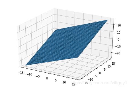
# 模型可视化
fig = plt.figure()
ax = Axes3D(fig)
X = np.arange(-15, 15, 0.25)
Y = np.arange(-15, 15, 0.25)
X, Y = np.meshgrid(X, Y) # x-y 平面的网格
Z = f(X, Y)
ax.plot_surface(X, Y, Z)
plt.show()
截距项:0.4932432432432401
系数:[0.90675676 0.91486486]
预测结果为:[3.22972973 5.04324324 4.14459459 5.05135135 5.95810811 6.87297297]
模型R^2= 0.9922372282300297
因为是随便造的数据,所以此处 R 2 R^2 R2非常高,模型非常之好。但是实际情况下的数据不会这么好, R 2 R^2 R2能到 0.7 0.7 0.7就不错了。
可以看出,模型其实是三维空间里的一个平面
关于评估模型
回归模型我们采用 R 2 R^2 R2来评估模型,更多评价指标,请看模型评估指标
均 方 误 差 = 1 n _ s a m p l e s ∑ i = 1 n _ s a m p l e s ( y _ t r u e − y _ p r e d ) 2 均方误差=\frac 1 {n\_samples} \sum_{i=1}^{n\_samples}(y\_true-y\_pred)^2 均方误差=n_samples1∑i=1n_samples(y_true−y_pred)2
R 2 = 1 − 均 方 误 差 v a r ( y _ t r u e ) R^2= 1 - \frac {均方误差}{var(y\_true)} R2=1−var(y_true)均方误差
梯度下降法
三种方法的优缺点:
- 批量梯度下降易于并行计算,但每次迭代计算所有样本,计算成本大
- 随机梯度下降一次迭代计算一个样本,计算量小,但迭代时样本是随机取,可能导致迭代次数变多
- 小批量梯度下降结合二者
批量梯度下降
import matplotlib.pyplot as plt
import numpy as np

# 准备数据
X = np.array([[1, 2], [3, 2], [1, 3], [2, 3], [3, 3], [3, 4]])
y = np.array([3.1, 5.1, 4.2, 5.2, 5.9, 6.8])
n_samples, n_features = X.shape
X = np.concatenate((np.ones(n_samples).reshape(
    (n_samples, 1)), X), axis=1)  # X添加一列1
y = y.reshape((n_samples, 1))

# 预定义超参数
alpha = 0.1  # 步长
max_iter = 1e6  # 最大迭代次数,防止模型发散,陷入死循环
epsilon = 1e-6  # 当前后两次迭代theta的变化小于epsilon则视为收敛,停止迭代,返回此时的theta
theta = np.zeros((n_features + 1, 1))  # 初始化theta
costs = []  # 用来存储每一次迭代时损失函数值的变化情况

# 定义损失函数
def cost_function(X, y, theta, n_samples):
    """损失函数"""
    return (X @ theta - y).T @ (X @ theta - y) / 2 / n_samples

# 迭代求解
for iter in range(int(max_iter)):
    theta_next = theta - alpha * (X.T) @ (X@theta - y) / n_samples
    cost = cost_function(X, y, theta, n_samples)[0][0]
    costs.append(cost)
    if np.abs(theta - theta_next).sum() < epsilon:
        theta = theta_next
        print("merge")  # 收敛
        break
    theta = theta_next
else:
    print("get the max_iter, stop iter.")

# 求出参数
intercept = theta[0, 0]
coef = theta[1:, 0]
print("截距项:%s" % intercept)
print("系数:%s" % coef)

# 可视化迭代过程中损失函数值的变化情况
plt.plot(list(range(len(costs))), costs)
plt.xlabel("iter count")
plt.ylabel("cost function")
plt.show()
输出:
merge
截距项:0.4930883696433331
系数:[0.90676633 0.91490961]

正规方程法求解出来的结果:
- 截距项:0.4932432432432401
- 系数:[0.90675676 0.91486486]
批量梯度下降法求解出来的结果:
- 截距项:0.4930883696433331
- 系数:[0.90676633 0.91490961]
可以看出,二者结果几乎相等,这点误差还是允许的。
模型一开始迭代,损失函数值就迅速下降,再往后就几乎不怎么变化了。
随机梯度下降
import matplotlib.pyplot as plt
import numpy as np

X = np.array([[1, 2], [3, 2], [1, 3], [2, 3], [3, 3], [3, 4]])
y = np.array([3.1, 5.1, 4.2, 5.2, 5.9, 6.8])
n_samples, n_features = X.shape
X = np.concatenate((np.ones(n_samples).reshape(
    (n_samples, 1)), X), axis=1)  # X添加一列1
y = y.reshape((n_samples, 1))

alpha = 0.1  # 步长
max_iter = 1e6  # 最大迭代次数,防止模型发散,陷入死循环
epsilon = 1e-6  # 当前后两次迭代theta的变化小于epsilon则视为收敛,停止迭代,返回此时的theta
theta = np.zeros((n_features + 1, 1))  # 初始化theta
costs = []  # 用来存储每一次迭代时损失函数值的变化情况

for iter in range(int(max_iter)):
    index = np.random.choice(n_samples, 1)  # 从0~n_samples-1随机取一个索引
    X_sample, y_sample = X[index], y[index]
    theta_next = theta - alpha * np.dot(X_sample.T, np.dot(X_sample, theta) - y_sample) / n_samples

    cost = cost_function(X, y, theta, n_samples)[0][0]
    costs.append(cost)
    if np.abs(theta - theta_next).sum() < epsilon:
        print('merge')
        theta = theta_next
        break
    theta = theta_next
else:
    print("get the max_iter, stop iter.")

intercept = theta[0, 0]
coef = theta[1:, 0]
print("截距项:%s" % intercept)
print("系数:%s" % coef)

plt.plot(list(range(len(costs))), costs)
plt.xlabel("iter count")
plt.ylabel("cost function")
输出:
merge
截距项:0.47652714599601687
系数:[0.90629319 0.90153283]

和上边的方法结果几乎一致,误差可忽略。结果略微震荡,是随机选择样本的缘故
小批量梯度下降
import matplotlib.pyplot as plt
import numpy as np

X = np.array([[1, 2], [3, 2], [1, 3], [2, 3], [3, 3], [3, 4]])
y = np.array([3.1, 5.1, 4.2, 5.2, 5.9, 6.8])
n_samples, n_features = X.shape
X = np.concatenate((np.ones(n_samples).reshape(
    (n_samples, 1)), X), axis=1)  # X添加一列1
y = y.reshape((n_samples, 1))

alpha = 0.1  # 步长
max_iter = 1e6  # 最大迭代次数,防止模型发散,陷入死循环
epsilon = 1e-4  # 当前后两次迭代theta的变化小于epsilon则视为收敛,停止迭代,返回此时的theta
batch_size = 3 # 每次挑选3个样本迭代
theta = np.zeros((n_features + 1, 1))  # 初始化theta
costs = []  # 用来存储每一次迭代时损失函数值的变化情况

for iter in range(int(max_iter)):
    index = np.random.choice(n_samples, batch_size)
    X_sample = X[index]
    y_sample = y[index]
    theta_next = theta - alpha * np.dot(X_sample.T, np.dot(X_sample, theta) - y_sample) / batch_size

    cost = cost_function(X, y, theta, n_samples)[0][0]
    costs.append(cost)
    if np.abs(theta - theta_next).sum() < epsilon:
        print('merge')
        theta = theta_next
        break
    theta = theta_next
else:
    print("get the max_iter, stop iter.")

intercept = theta[0, 0]
coef = theta[1:, 0]
print("截距项:%s" % intercept)
print("系数:%s" % coef)

plt.plot(list(range(len(costs))), costs)
plt.xlabel("iter count")
plt.ylabel("cost function")
merge
截距项:0.49515442857645536
系数:[0.90220847 0.8995099 ]

和上边的方法结果几乎一致,误差可忽略。结果略微震荡,是随机选择样本的缘故