【CS229 lecture18】linear quadratic regulation(LQR) 线性二次型调节控制

lecture18
今天来讨论我最喜欢的算法之一，用以控制MDP，我觉得是一个优雅、高效、强大的算法。先讨论MDP的几个常见变种（与现有的MDP定义会有不同）。

---

Agenda
state-action rewards
finite horizon MDPs
linear dynamical systems 线性动力系统
-models
-linear quadratic regulation(LQR) 线性二次型调节控制

---

just a recap：MDP is a five tuple(下图给出一般性的定义，然后做一些改动，生成variations)

---

---

首先在reward function上做一些改动，使之不仅仅是states的函数，而且还是action的函数。记得在上一讲时，我说过对于无限连续状态的MDP，不能直接应用value iteration，因为对于continuous MDP, we use some approximations of the optimal value function. But later, we’ll talk about a special case of MDPs, where you can actually represent the value function exactly, even if you have an infinite-state space or even if you have a continuous-state space. I’ll actually do that, talk about these special constants of infinite-state MDPs, using this new variations of the reward function and the alternative to just counting, so start to make the formulation a little easier.

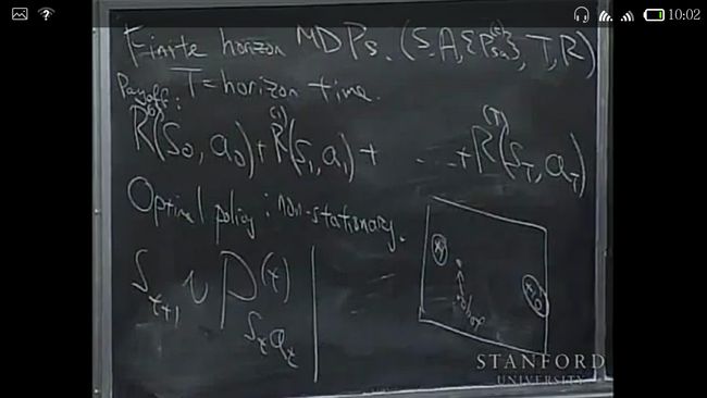
first variation: state-action reward 比如机器人动起来比静止麻烦，所以reward和action也有关系了。

---

---

second variation: finite horizon MDP
图中说到的optimal policy may be non-stationery（非平稳的），that is to say, my optimal action to take will be different for different time steps. 然后举了一个例子（见黑板右下的方框内）
Since we have non-stationery optimal policy ，I’m going to allow non-stationery transition probabilities （非平稳过渡概率）as well. 比如说飞机，飞久了燃料就少了，转移概率就是时变的。

---

---

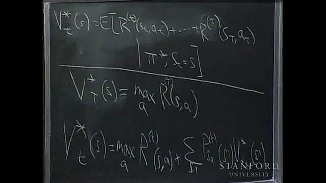
So now we have a non-stationery optimal policy, let’s talk about an algorithm to actually try to find the optimal policy. Let’s define the following.(图中的value function start increasingly from time t and end at time T), and write out the value iteration algorithm（横线下面）.
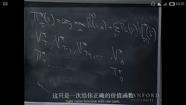
事实上，有一个很漂亮的dynamics programming algorithm(动态规划算法)来解决，从T开始，反向计算。

---

---

有人提问，finite horizon MDP 没有了discounting 那一项，也就是γ（用以调节reward随时间衰减的）
Andrew: usually use either finite horizon MDP or discounting, not the both. 其实二者在作用上又一些共同，都可以保证value function 是有限的。
以上就是finite horizon MDP

---

下面综合以上两种idea来提出一种special MDP（虽然有着strong assumptions , but are reasonable），along with a very elegant and effective algorithm to solve the even very large MDP.

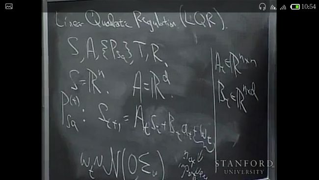
LQR
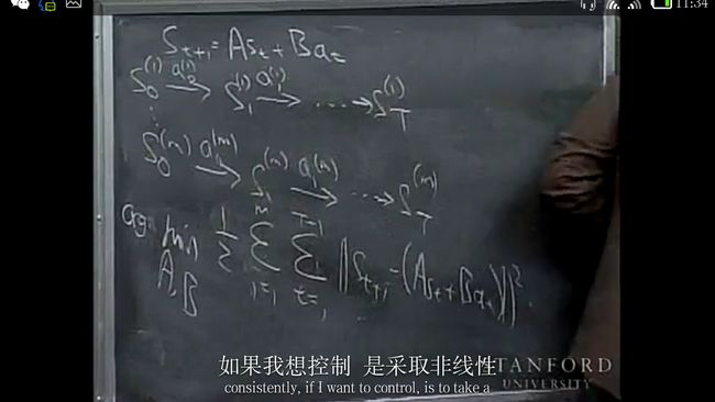
要用到和finite horizon MDP 一样的动态规划算法。specify the problem first, assume A B W are given, our goal is to find an optimal policy. 另外，图中的noise （W）其实并不重要，所以后面的可能会忽略，或者处理的比较马虎。

---

---

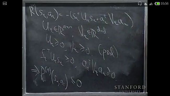
assume Ut and Vt are positive semi definite（半正定的），从而reward 函数总是负的。

---

---

对于以上，for a complete example（以便理解）, suppose you have a helicopter : want St 尽可能等于0

---

---

接下来的几个步骤 I’m going to derive things for the general case of non-stationary dynamics（非稳态动力学），会有更多的数学和equations for LQR, I’m going to write out the case for the fairy general case of time varied dynamics and time varied reward functions.为了便于理解，你们可以忽略一些带有时间下标的符号，假想是固定的。
然后会讲extension of this called differential dynamic programming（微分动态规划的扩展）

先讲一下how to come up with a linear model. The key assumption in the model is that the dynamics are linear. There is also the assumption that reward function is quadratic.
If you have an inverted pendulum system, and you want to model the inverted pendulum using a linear model like this…

---

---

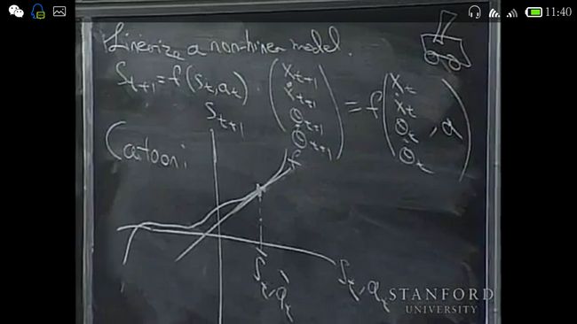
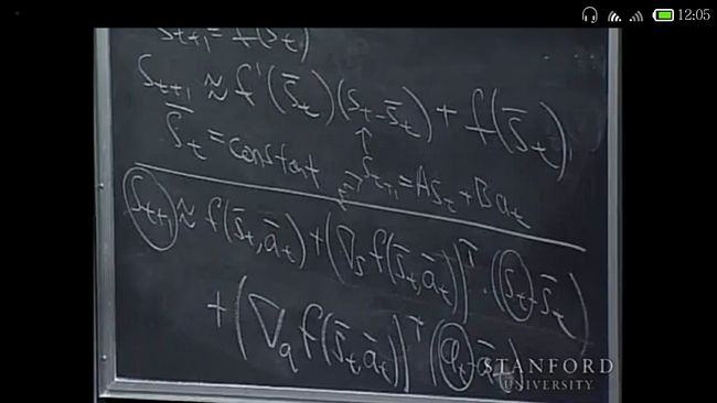
another way to come up with a linear model is to linearize a nonlinear model.（需要注意的问题是：应该在期望工作点附近线性化，比如倒立摆的竖直位置，否则远端的误差太大了。）

---

---

write it(linearize a nonlinear model)in math, first write the simple case and the fully general one in a second.

---

---

now I’ll post a LQR problem, given A B U V, then our goal is to come up with a policy to maximize the expected value of this rewards.
算法正是早先提到的用于解决 finite horizon 的动态规划算法。
下图中的（because …≥0）是因为VT矩阵是半正定的，最后时刻T肯定希望没有动作。

---

---

好了，现在让我们做动态规划的步骤(DP steps)：简单说就是given V*t+1想要求V*t

---

---

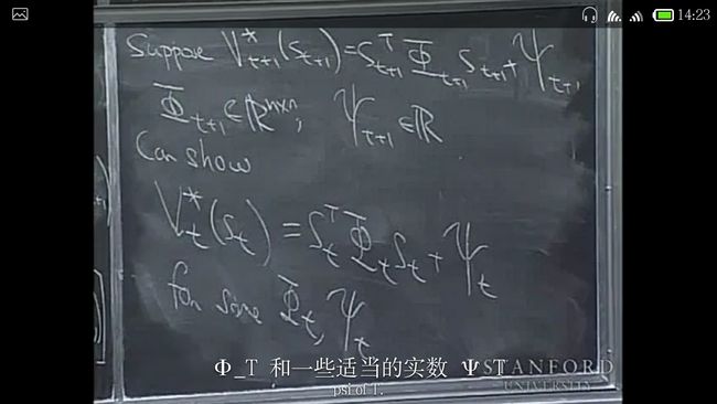
It turns out LQR has following useful property, it turns out each of these value function can be represented as a quadratic function . （不理解？？）

---

---

所以你可以这样开始递归

---

---

St状态的value function 等于t时刻的即时reward和St+1时刻的reward的期望。。。

---

对at求导可得optimal action(some linear combination of states St，或者一个矩阵Lt乘以St)

---

---

然后把at放回去，做maximization，你会得到这个，其中迭代公式的名称叫做Discrete time Riccati equatoin ：

---

---

So, to summarize, our algorithm for finding the exact solution to finite horizon LQR problems is as follows.

---

---

Andrew在总结时的一段话：
So the very cool thing about the solution of discrete time LQR problems finite horizon LQR problems is that this is a problem in an infinite state, with a continuous state. But nonetheless, under the assumptions we made, you can prove that the value function is a quadratic function of the state. Therefore, just by computing these matrixes phi(t) and the real number psi(t), you can actually exactly represent the value function, even for these infinite large state spaces, even for continuous state spaces. And so the computation of these algorithms scales only like the cubes, scales only as a polynomial in terms of the number of state variables… it’s easily applied to problems with even very large states spaces, so we actually often apply variations of this algorithm to some subset, to some particular subset for the things we do on our helicopter, which has high dimensional state spaces with twelve or higher dimensions. This has worked very well for that.
So it turns out there are even more things you can do with this…
关于这个还有一些很精妙的结论，下讲我再讲。

---