机器学习系列笔记十二: 决策树
机器学习系列笔记十二: 决策树
文章目录
- 机器学习系列笔记十二: 决策树
- Intro
- 信息熵
- 使用信息熵寻找最优划分
- 基尼系数
- 使用基尼系数寻找最佳划分
- 基尼系数与信息熵的对比
- CART与决策树中的超参数
- 决策树的超参数
- 决策树解决回归问题
- 决策树的局限性
- 缺点
- 改进措施
- 总结
- 参考致谢
Intro
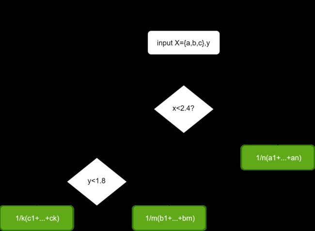
以招聘机器学习算法工程师为例子,对于一个应聘者的信息输入,决策的流程可以一个树结构来表示:

通过多级判断产生多个判断条件作为根节点,多个结果作为叶子节点,这样的过程就叫做决策树。通常我们把决策树的深度定义为获取最终结果的最大所需判断数。在上图中,最多通过三次判断就能将样本(应聘者信息)进行相应的分类,所以该决策树的深度为3.
以使用决策树对鸢尾花分类所得到的决策边界为例:
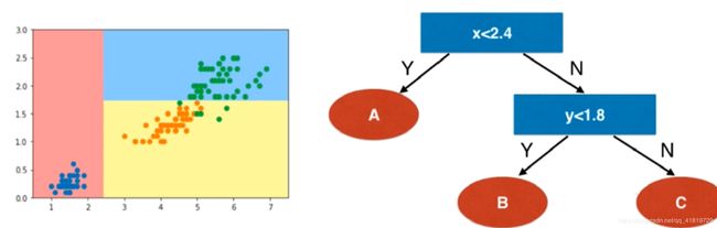
在每一个节点上选择每一个维度以及该维度相应的一个阈值,过程类似于OvR,每次都得出一个分类结果,最后得到所有分类结果。
什么是决策树
- 非参数学习算法
- 可以解决分类问题
- 天然可以解决多分类问题
- 也可以解决回归问题
- 非常好的可解释性
构建决策树的关键问题
根节点是判断条件:if var(左半部分) > val(右半部分)
-
每个根节点在哪个样本特征维度做划分,换言之各个根节点判断条件左半部分怎么设定
-
某个维度在哪个阈值上做划分,换言之判断条件的右半部分如何设定
信息熵
信息熵在信息论中表示随机变量不确定度的度量,在信息论中认为不确定性越低的信息包含的信息量(信息熵)越大。
- 熵越大,数据的不确定性越高
- 熵越小,数据的不确定性越低
熵的计算公式如下:
H = − ∑ i = 1 k p i l o g ( p i ) H=-\sum^k_{i=1}p_ilog(p_i) H=−i=1∑kpilog(pi)
对于只有p1–>A类,p2–>B类,该函数的图像如下:
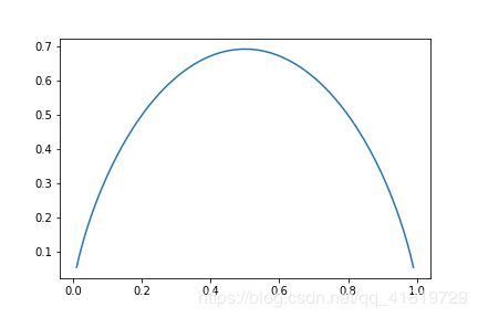
可以看到,当样本是A类或B类相等=0.5时,此时该样本的不确定性最大,信息熵也为最大。
通过对信息熵的使用,可以解决构建决策树的关键问题:对所有的可能划分进行搜索,找到一个最好的划分,使得划分后信息熵最小。
使用信息熵寻找最优划分
使用scikit learn的决策树分类算法
import numpy as np
import matplotlib.pyplot as plt
from sklearn import datasets
from sklearn.tree import DecisionTreeClassifier
import warnings

warnings.filterwarnings("ignore")

iris = datasets.load_iris()
X = iris.data[:,2:]
y = iris.target
# 使用决策树分类器
dt_clf = DecisionTreeClassifier(max_depth=2,criterion="entropy")
dt_clf.fit(X,y)
DecisionTreeClassifier(class_weight=None, criterion='entropy', max_depth=2,
                       max_features=None, max_leaf_nodes=None,
                       min_impurity_decrease=0.0, min_impurity_split=None,
                       min_samples_leaf=1, min_samples_split=2,
                       min_weight_fraction_leaf=0.0, presort=False,
                       random_state=None, splitter='best')
绘制决策边界
def plot_decision_boundary(model,axis):
    x0,x1 = np.meshgrid(
        np.linspace(axis[0],axis[1],int((axis[1]-axis[0])*100)).reshape(-1,1),
        np.linspace(axis[2],axis[3],int((axis[3]-axis[2])*100)).reshape(-1,1),
    )
    X_new = np.c_[x0.ravel(),x1.ravel()]
    y_predict = model.predict(X_new)
    zz = y_predict.reshape(x0.shape)
    from matplotlib.colors import ListedColormap
    custom_cmap = ListedColormap(['#EF9A9A','#FFF59D','#90CAF9'])
    plt.contourf(x0,x1,zz,linewidth=5,cmap=custom_cmap)
plot_decision_boundary(dt_clf,axis=[0.5,7.5,0,3])
plt.scatter(X[y==0,0],X[y==0,1])
plt.scatter(X[y==1,0],X[y==1,1])
plt.scatter(X[y==2,0],X[y==2,1])
plt.show()

模拟使用信息熵进行划分
from collections import Counter
from math import log
def entropy(y):
    counter=Counter(y)
    res = 0.0
    for num in counter.values():
        p = num / len(y)
        res += -p * log(p)
    return res
def split(X,y,d,value):
    """基于维度d与阈值value进行划分"""
    index_a = (X[:,d]<=value)
    index_b = (X[:,d]>value)
    return X[index_a],X[index_b],y[index_a],y[index_b]
def try_split(X,y):
    """寻找最佳划分"""
    best_entropy = float("inf")
    best_d,best_v = -1,-1
    for d in range(X.shape[1]):
        # 可选的阈值是维度d下每两个特征的均值
        sorted_index = np.argsort(X[:,d])
        for i in range(1,len(X)):
            if X[sorted_index[i-1],d]!=X[sorted_index[i],d]:
                v = (X[sorted_index[i-1],d]+X[sorted_index[i],d])/2
                x_L,x_r,y_L,y_r=split(X,y,d,v)
                e = entropy(y_L)+entropy(y_r)
                if e < best_entropy:
                    best_entropy,best_d,best_v=e,d,v
    return best_entropy,best_d,best_v
best_entropy,best_d,best_v = try_split(X,y)
print("best_entropy:",best_entropy)
print("best_d:",best_d)
print("best_v:",best_v)
best_entropy: 0.6931471805599453
best_d: 0
best_v: 2.45
对照前面绘制的决策边界,可以看到第0个维度(x轴)的2.45进行划分是符合期待的
X1_L,X1_r,y1_L,y1_r = split(X,y,best_d,best_v)
entropy(y1_L)
0.0
entropy(y1_r)
0.6931471805599453
可以看到对于X1_L已经不需要进行划分了,其信息熵为0,但是对于右边X1_r,我们还需要再进行划分
best_entropy2,best_d2,best_v2 =try_split(X1_r,y1_r)
print("best_entropy:",best_entropy2)
print("best_d:",best_d2)
print("best_v:",best_v2)
best_entropy: 0.4132278899361904
best_d: 1
best_v: 1.75
对比决策边界图,可以看到在y轴(第二个维度)的1.75(阈值)进行划分是符合模拟结果的
X2_L,X2_r,y2_L,y2_r = split(X1_r,y1_r,best_d2,best_v2)
entropy(y2_L)
0.30849545083110386
entropy(y2_r)
0.10473243910508653
基尼系数
定义:
G = 1 − ∑ i = 1 k p i 2 G=1-\sum^k_{i=1}p_i^2 G=1−i=1∑kpi2
基尼系数和信息熵在决策树中的作用基本一致,都是用于度量数据的确定性的。
- 基尼系数越高,意味着数据的随机性越高
- 基尼系数越低,意味着数据的确定性越高
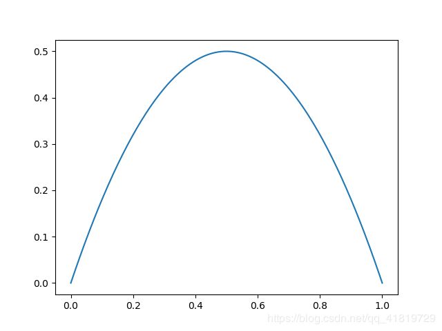
对于二分类的样本,其基尼系数可以表征为:
G = 1 − x 2 − ( 1 − x ) 2 = − 2 x 2 + 2 x G=1-x^2-(1-x)^2\\ =-2x^2+2x G=1−x2−(1−x)2=−2x2+2x
其函数图像如下:
使用基尼系数寻找最佳划分
在使用决策树分类器的时候将搜索划分维度与阈值的评判标准设置为criterion="gini"
import numpy as np
import matplotlib.pyplot as plt
from sklearn import datasets
from sklearn.tree import DecisionTreeClassifier
import warnings
warnings.filterwarnings("ignore")
iris = datasets.load_iris()
X = iris.data[:,2:]
y = iris.target

dt_clf = DecisionTreeClassifier(max_depth=2,criterion="gini")
dt_clf.fit(X,y)
DecisionTreeClassifier(class_weight=None, criterion='gini', max_depth=2,
                       max_features=None, max_leaf_nodes=None,
                       min_impurity_decrease=0.0, min_impurity_split=None,
                       min_samples_leaf=1, min_samples_split=2,
                       min_weight_fraction_leaf=0.0, presort=False,
                       random_state=None, splitter='best')
同样,绘制决策边界
def plot_decision_boundary(model,axis):
    x0,x1 = np.meshgrid(
        np.linspace(axis[0],axis[1],int((axis[1]-axis[0])*100)).reshape(-1,1),
        np.linspace(axis[2],axis[3],int((axis[3]-axis[2])*100)).reshape(-1,1),
    )
    X_new = np.c_[x0.ravel(),x1.ravel()]
    y_predict = model.predict(X_new)
    zz = y_predict.reshape(x0.shape)
    from matplotlib.colors import ListedColormap
    custom_cmap = ListedColormap(['#EF9A9A','#FFF59D','#90CAF9'])
    plt.contourf(x0,x1,zz,linewidth=5,cmap=custom_cmap)

plot_decision_boundary(dt_clf,axis=[0.5,7.5,0,3])
plt.scatter(X[y==0,0],X[y==0,1])
plt.scatter(X[y==1,0],X[y==1,1])
plt.scatter(X[y==2,0],X[y==2,1])
plt.show()

模拟使用基尼系数划分
from collections import Counter
from math import log
def gini(y):
    counter=Counter(y)
    res = 1.0
    for num in counter.values():
        p = num / len(y)
        res -= p ** 2
    return res

def split(X,y,d,value):
    """基于维度d与阈值value进行划分"""
    index_a = (X[:,d]<=value)
    index_b = (X[:,d]>value)
    return X[index_a],X[index_b],y[index_a],y[index_b]

def try_split(X,y):
    """寻找最佳划分"""
    best_g = float("inf")
    best_d,best_v = -1,-1
    for d in range(X.shape[1]):
        # 可选的阈值是维度d下每两个特征的均值
        sorted_index = np.argsort(X[:,d])
        for i in range(1,len(X)):
            if X[sorted_index[i-1],d]!=X[sorted_index[i],d]:
                v = (X[sorted_index[i-1],d]+X[sorted_index[i],d])/2
                x_L,x_r,y_L,y_r=split(X,y,d,v)
                g = gini(y_L)+gini(y_r)
                if g < best_g:
                    best_g,best_d,best_v=g,d,v

    return best_g,best_d,best_v
best_g,best_d,best_v = try_split(X,y)
print("best_g:",best_g)
print("best_d:",best_d)
print("best_v:",best_v)
best_g: 0.5
best_d: 0
best_v: 2.45
X1_L,X1_r,y1_L,y1_r = split(X,y,best_d,best_v)
print("gini of y1_L:",gini(y1_L))
print("gini of y1_r:",gini(y1_r))
gini of y1_L: 0.0
gini of y1_r: 0.5
best_g2,best_d2,best_v2 =try_split(X1_r,y1_r)
print("best_g2:",best_g2)
print("best_d2:",best_d2)
print("best_v2:",best_v2)
best_g2: 0.2105714900645938
best_d2: 1
best_v2: 1.75
X2_L,X2_r,y2_L,y2_r = split(X1_r,y1_r,best_d2,best_v2)
print("gini of y2_L:",gini(y2_L))
print("gini of y2_r:",gini(y2_r))
gini of y2_L: 0.1680384087791495
gini of y2_r: 0.04253308128544431
基尼系数与信息熵的对比
由二者的计算公式可以看出,信息熵的计算(log)是比基尼系数(平方)稍慢的,所以scikit-learn中默认为基尼系数,
大多数时候二者没有特别的效果优劣。
CART与决策树中的超参数
CART全称为Classification And Regression Tree,是根据某一个维度d和某一个阈值v进行二分所形成的决策二叉树。在scikit-learn中的决策树实现就是CART.
其余的决策树ID3 ,C4.5,C5.0
对于通过CART实现的决策树,其复杂度分别为:
-
预测:
O(logm) -
训练:
O(n*m*logm)
可以看到CART模型的训练复杂度相当高,这是因为每次寻找划分都要遍历所有样本,与knn类似,同时极其容易产生过拟合,那么有什么方法可以降低复杂度并且解决过拟合问题呢?剪枝!
而剪枝就涉及到了许多决策树的超参数,在scikit-learn中我们可以通过调节这些超参数来完成对CART的剪枝,减少模型的过拟合。
决策树的超参数
import numpy as np
import matplotlib.pyplot as plt
from sklearn import datasets
import warnings
warnings.filterwarnings("ignore")
X,y = datasets.make_moons(noise=0.25,random_state=666)
plt.scatter(X[y==0,0],X[y==0,1])
plt.scatter(X[y==1,0],X[y==1,1])
plt.show()

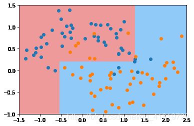
创建默认参数的决策树模型,不指定depth,模型在训练时会使得划分的各部分数据基尼值为0
from sklearn.tree import DecisionTreeClassifier

dt_clf = DecisionTreeClassifier()
dt_clf.fit(X,y)
DecisionTreeClassifier(class_weight=None, criterion='gini', max_depth=None,
                       max_features=None, max_leaf_nodes=None,
                       min_impurity_decrease=0.0, min_impurity_split=None,
                       min_samples_leaf=1, min_samples_split=2,
                       min_weight_fraction_leaf=0.0, presort=False,
                       random_state=None, splitter='best')
绘制决策边界
def plot_decision_boundary(model,axis):
    x0,x1 = np.meshgrid(
        np.linspace(axis[0],axis[1],int((axis[1]-axis[0])*100)).reshape(-1,1),
        np.linspace(axis[2],axis[3],int((axis[3]-axis[2])*100)).reshape(-1,1),
    )
    X_new = np.c_[x0.ravel(),x1.ravel()]
    y_predict = model.predict(X_new)
    zz = y_predict.reshape(x0.shape)
    from matplotlib.colors import ListedColormap
    custom_cmap = ListedColormap(['#EF9A9A','#FFF59D','#90CAF9'])
    plt.contourf(x0,x1,zz,linewidth=5,cmap=custom_cmap)

plot_decision_boundary(dt_clf,axis=[-1.5,2.5,-1,1.5])
plt.scatter(X[y==0,0],X[y==0,1])
plt.scatter(X[y==1,0],X[y==1,1])
plt.scatter(X[y==2,0],X[y==2,1])
plt.show()
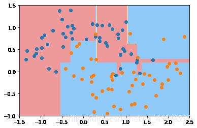
该决策边界极其不规则,显然出现了过拟合
超参数:决策树深度max_depth
dt_clf2 = DecisionTreeClassifier(max_depth=2)
dt_clf2.fit(X,y)
plot_decision_boundary(dt_clf2,axis=[-1.5,2.5,-1,1.5])
plt.scatter(X[y==0,0],X[y==0,1])
plt.scatter(X[y==1,0],X[y==1,1])
plt.scatter(X[y==2,0],X[y==2,1])
plt.show()
可以看到通过调整max-depth有效缓解了模型的过拟合
超参数:节点划分所需的最小样本数min_samples_split
dt_clf3 = DecisionTreeClassifier(min_samples_split=10)
dt_clf3.fit(X,y)
plot_decision_boundary(dt_clf3,axis=[-1.5,2.5,-1,1.5])
plt.scatter(X[y==0,0],X[y==0,1])
plt.scatter(X[y==1,0],X[y==1,1])
plt.scatter(X[y==2,0],X[y==2,1])
plt.show()
min_sample_split越大,模型复杂度越低,越不容易出现过拟合
超参数:叶子节点拥有的最小样本数min_samples_leaf
dt_clf4 = DecisionTreeClassifier(min_samples_leaf=6)
dt_clf4.fit(X,y)
plot_decision_boundary(dt_clf4,axis=[-1.5,2.5,-1,1.5])
plt.scatter(X[y==0,0],X[y==0,1])
plt.scatter(X[y==1,0],X[y==1,1])
plt.scatter(X[y==2,0],X[y==2,1])
plt.show()
min_samples_leaf的设置越大,越容易出现欠拟合,同时减少过拟合的程度
超参数:最大叶子节点数max_leaf_nodes
dt_clf5 = DecisionTreeClassifier(max_leaf_nodes=4)
dt_clf5.fit(X,y)
plot_decision_boundary(dt_clf5,axis=[-1.5,2.5,-1,1.5])
plt.scatter(X[y==0,0],X[y==0,1])
plt.scatter(X[y==1,0],X[y==1,1])
plt.scatter(X[y==2,0],X[y==2,1])
plt.show()

max_leaf_nodes越小,剪的枝越多,越抑制过拟合
决策树解决回归问题
将决策树的叶节点中存储的数据均值作为该叶节点的值,就可以通过决策树解决回归问题。
决策树解决分类问题的实验
使用波士顿房价数据集
import numpy as np
import matplotlib.pyplot as plt
import warnings
from sklearn import datasets
from sklearn.model_selection import train_test_split
warnings.filterwarnings("ignore")

boston = datasets.load_boston()
X = boston.data
y = boston.target
X_train,X_test,y_train,y_test = train_test_split(X,y)
使用Decision Tree Regressor
from sklearn.tree import DecisionTreeRegressor

dt_reg = DecisionTreeRegressor()
dt_reg.fit(X_train,y_train)
DecisionTreeRegressor(criterion='mse', max_depth=None, max_features=None,
                      max_leaf_nodes=None, min_impurity_decrease=0.0,
                      min_impurity_split=None, min_samples_leaf=1,
                      min_samples_split=2, min_weight_fraction_leaf=0.0,
                      presort=False, random_state=None, splitter='best')
dt_reg.score(X_test,y_test)
0.7977702945741157
dt_reg.score(X_train,y_train)
1.0
可以看到在训练集上预测的准确率为100%,而在测试集中却只有80%,这显然是出现了过拟合。
我们可以通过调整超参数来改进模型
dt_reg = DecisionTreeRegressor(max_depth=11)
dt_reg.fit(X_train,y_train)
test_score = dt_reg.score(X_test,y_test)
train_score = dt_reg.score(X_train,y_train)
print("test score:",test_score)
print("train score:",train_score)
test score: 0.8143530281488656
train score: 0.9966466937009163
dt_reg = DecisionTreeRegressor(min_samples_split=20)
dt_reg.fit(X_train,y_train)
test_score = dt_reg.score(X_test,y_test)
train_score = dt_reg.score(X_train,y_train)
print("test score:",test_score)
print("train score:",train_score)
test score: 0.819273046898797
train score: 0.9395914308946647
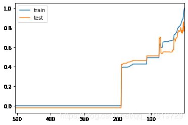
我们可以通过绘制模型复杂度曲线来观察超参数对模型拟合度的影响情况
from sklearn.tree import DecisionTreeRegressor
from sklearn.metrics import r2_score

maxSampleLeaf = 506
train_scores = []
test_scores = []
for i in range(1, maxSampleLeaf+1):
    dt_reg = DecisionTreeRegressor(min_samples_leaf=i)
    dt_reg.fit(X_train, y_train)
    y_train_predict = dt_reg.predict(X_train)
    train_scores.append(r2_score(y_train, y_train_predict))
    test_scores.append(dt_reg.score(X_test, y_test))

plt.plot([i for i in range(1, maxSampleLeaf+1)], train_scores, label="train")
plt.plot([i for i in range(1, maxSampleLeaf+1)], test_scores, label="test")
plt.xlim(506, 1)
plt.legend()
plt.show()
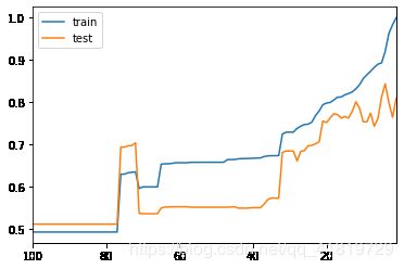
maxSampleLeaf = 100
train_scores = []
test_scores = []
for i in range(1, maxSampleLeaf+1):
    dt_reg = DecisionTreeRegressor(min_samples_leaf=i)
    dt_reg.fit(X_train, y_train)
    y_train_predict = dt_reg.predict(X_train)
    train_scores.append(r2_score(y_train, y_train_predict))
    test_scores.append(dt_reg.score(X_test, y_test))

plt.plot([i for i in range(1, maxSampleLeaf+1)], train_scores, label="train")
plt.plot([i for i in range(1, maxSampleLeaf+1)], test_scores, label="test")
plt.xlim(maxSampleLeaf, 1)
plt.legend()
plt.show()
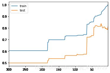
maxSamplesSplit = 300
train_scores = []
test_scores = []
for i in range(2, maxSamplesSplit+1):
    dt_reg = DecisionTreeRegressor(min_samples_split=i)
    dt_reg.fit(X_train, y_train)
    y_train_predict = dt_reg.predict(X_train)
    train_scores.append(r2_score(y_train, y_train_predict))
    test_scores.append(dt_reg.score(X_test, y_test))

plt.plot([i for i in range(2, maxSamplesSplit+1)], train_scores, label="train")
plt.plot([i for i in range(2, maxSamplesSplit+1)], test_scores, label="test")
plt.xlim(maxSamplesSplit, 2)
plt.legend()
plt.show()
决策树的局限性
决策树的优势:
1、便于理解和解释。树的结构可视化
2、训练需要的数据少,其他机器学习模型通常需要数据规范化,比如构建虚拟变量和移除缺失值
3、由于训练决策树的数据点的数量导致了决策树的使用开销呈指数分布(训练树模型的时间复杂度是参加训练数据点的对数值)
4、能够处理数值型数据和分类数据,其他的技术通常只能用来专门分析某一种的变量类型的数据集;
5、能够处理多路输出问题;
6、使用白盒模型。如果某种给定的情况在模型中是可以观察的,那么就可以轻易的通过布尔逻辑来解释这种情况,相比之下在黑盒模型中的结果就是很难说明清楚了;
7、可以通过数值统计测试来验证该模型。这对解释验证该模型的可靠性成为可能
8、即使是该模型假设的结果越真实模型所提供的数据有些违反,其表现依旧良好
决策树的缺点:
1、决策树模型容易产生一个过于复杂的模型,这样的模型对数据的泛化性能会很差。这就是所谓的过拟合,一些策略像剪枝、设置叶节点所需要的最小样本数或者设置数的最大深度就是避免出现该问题的最有效的方法。(剪枝:在机器学习经典算法中,决策树算法的重要性想必大家都是知道的。不管是ID3算法还是比如C4.5算法等等,都面临一个问题,就是通过直接生成的完全决策树对于训练样本来说是“过度拟合”的,说白了是太精确了。由于完全决策树对训练样本的特征描述得“过于精确” ,无法实现对新样本的合理分析, 所以此时它不是一棵分析新数据的最佳决策树。解决这个问题的方法就是对决策树进行剪枝,剪去影响预测精度的分支。常见的剪枝策略有预剪枝(pre -pruning)技术和后剪枝(post -pruning )技术两种。预剪枝技术主要是通过建立某些规则限制决策树的充分生长, 后剪枝技术则是待决策树充分生长完毕后再进行剪枝。)
2、决策树可能是不稳定的,因为在数据中的微小变化可能会导致完全不同的树生成。这个问题可以通过决策树的集成来得到缓解;
3、在多方面性能最优和简单化概念的要求下,学习一颗最优决策树通常是一个NP难问题 ,因此,实际的决策树学习算法是基于启发式算法,例如在每个节点进行局部最优决策的贪心算法,这样的算法不能保证返回全局最有决策树,这个问题可以通过集成学习来训练多颗决策树来缓解,这多棵决策树一般通过对特征和样本又放回的随机采样来生成;
4、有些概念很难被决策树学习到,因为决策树很难清楚的表述那些概念,例如XOR,奇偶或者复用器问题;
5、如果某些类在问题中占主导地位会使得创始的决策树有偏差,因此建议在拟合前先对数据集进行平衡。
缺点
容易发生过拟合(随机森林可以很大程度上减少过拟合),如下图所示

并查集的局限性(决策树算法对个别数据敏感)
import numpy as np
import matplotlib.pyplot as plt
from sklearn import datasets
from sklearn.tree import DecisionTreeClassifier
import warnings
warnings.filterwarnings("ignore")

iris = datasets.load_iris()
X=iris.data[:,2:]
y = iris.target
dt_clf = DecisionTreeClassifier(max_depth=2,criterion="entropy")
dt_clf.fit(X,y)
def plot_decision_boundary(model,axis):
    x0,x1 = np.meshgrid(
        np.linspace(axis[0],axis[1],int((axis[1]-axis[0])*100)).reshape(-1,1),
        np.linspace(axis[2],axis[3],int((axis[3]-axis[2])*100)).reshape(-1,1),
    )
    X_new = np.c_[x0.ravel(),x1.ravel()]
    y_predict = model.predict(X_new)
    zz = y_predict.reshape(x0.shape)
    from matplotlib.colors import ListedColormap
    custom_cmap = ListedColormap(['#EF9A9A','#FFF59D','#90CAF9'])
    plt.contourf(x0,x1,zz,linewidth=5,cmap=custom_cmap)

plot_decision_boundary(dt_clf,axis=[0.5,7.5,0,3])
plt.scatter(X[y==0,0],X[y==0,1])
plt.scatter(X[y==1,0],X[y==1,1])
plt.scatter(X[y==2,0],X[y==2,1])
plt.show()
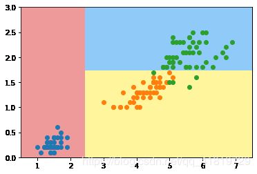
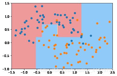
上图是原始数据集使用CART决策树算法得到的分类边界,现在我们要删除原数据集中的某一个样本删除
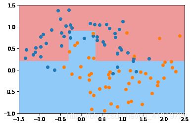
X_new = np.delete(X,138,axis=0)
y_new = np.delete(y,138)
dt_clf2 = DecisionTreeClassifier(max_depth=2,criterion="entropy")
dt_clf2.fit(X_new,y_new)
plot_decision_boundary(dt_clf2,axis=[0.5,7.5,0,3])
plt.scatter(X_new[y_new==0,0],X_new[y_new==0,1])
plt.scatter(X_new[y_new==1,0],X_new[y_new==1,1])
plt.scatter(X_new[y_new==2,0],X_new[y_new==2,1])
plt.show()

可以看到虽然只删除了一个样本,但是训练得到的决策边界/模型就完全不同了,这就说明了决策树对于个别样本点是很敏感的,这也是所有非参数学习算法的通病:高度依赖于原始数据,有很严重的过拟合倾向,需要调参进行优化。
改进措施
-
对决策树进行剪枝。可以采用交叉验证法和加入正则化的方法;
-
使用基于决策树的集成算法,如bagging算法,randomforest算法,可以解决过拟合的问题。
总结

参考致谢
liuyubobo:https://github.com/liuyubobobo/Play-with-Machine-Learning-Algorithms
liuyubobo:https://coding.imooc.com/class/169.html
维基百科:
决策树的优缺点:https://blog.csdn.net/weixin_41540084/article/details/99325672