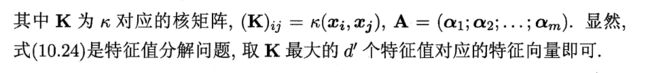
自己实现降维之核主成分分析(KPCA)
许多机器学习算法都假定输入数据是线性可分的。感知器为了保证其收敛性,甚至要求训练数据是完美线性可分的。然而,在现实世界中,大多数情况下我们面对的是非线性问题,针对此类问题,通过降维技术,如PCA和LDA等,将其转化为线性问题并不是最好的办法。
核函数与核技巧
其实很简单,就是将线性不可分的数据映射到更高维度上去使其线性可分。换句话说,利用核PCA,可以通过非线性映射将数据转换到一个高维空间,然后在此高维空间中使用标准PCA将其映射到另外一个低维空间中,并通过线性分类器进行划分(前提条件,样本可根据输入空间的密度进行划分)。但是,这种方法的确定是带来高昂的计算成本,这也是为什么要使用核技巧的原因。通过使用核技巧,可以在原始特征空间中计算两个高维特种空间中向量的相似度。
核PCA公式推导:
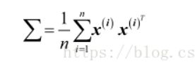
标准的PCA的协方差矩阵∑公式如下:
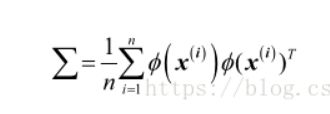
可以使用 ϕ (核函数)通过在原始特征空间上的非线性特征组合来替代样本间点积的计算:
接下来就是进行标准的PCA操作

将上述变换一下,得到特征向量

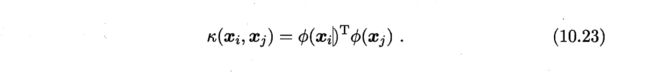
一般情形下,我们不清楚。的具体形式,于是引入核函数
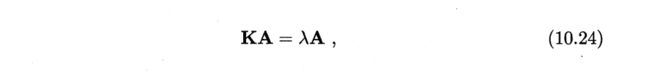
将式(10.22)和(10.23)代入式(10.21)后化简可得
常用的核函数有:


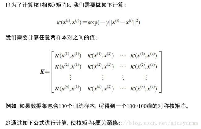
综上,由于测试需要这里来实现一个基于高斯核的PCA:
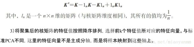
(也就是所谓的中心化核矩阵,具体为什么这样做就能中心化它,并没有研究过)
代码实现:
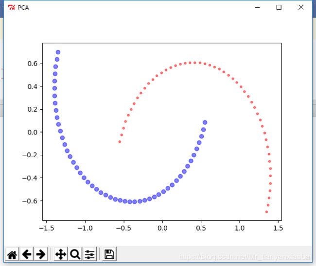
测试数据(这里用sklearn中的makemoon函数制造一个半月形的数据集)
import numpy as np
import matplotlib.pyplot as plt
import DownCompentTool as DT
#kpca测试
from sklearn.datasets import make_moons
tool = DT.down()
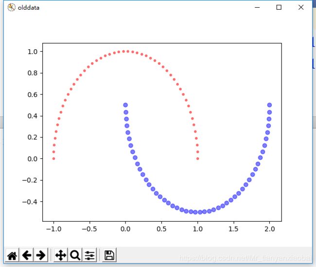
X, y = make_moons(n_samples=100, random_state=123)
plt.figure("olddata")
plt.scatter(X[y == 0, 0], X[y == 0, 1], color='red', marker='.', alpha=0.5)
plt.scatter(X[y == 1, 0], X[y == 1, 1], color='blue', marker='o', alpha=0.5)
如下图所示:
利用传统pca进行降维:
    def PCA_my(self, attributes, compents):
        #对x进行去中心化处理
        ss = StandardScaler()
        attributes = ss.fit_transform(attributes)

        #计算样本的协方差矩阵X*X(T)
        covx = np.dot(attributes,attributes.T)
        lamda, V = np.linalg.eigh(covx)
        index= np.argsort(-lamda)[:compents]
        diag_lamda = np.sqrt(np.diag(-np.sort(-lamda)[:compents]))
        # 取出对应的特征向量矩阵
        V_selected = V[:, index]
        Z = V_selected.dot(diag_lamda)
        print np.sum(V_selected)
        return Z
    def PCA_sk(self, attributes, compents):
        from sklearn.decomposition import PCA
        pca = PCA(n_components=compents)
        newX = pca.fit_transform(attributes)
        return  newX

    def rbf_kernel_PCA_my(self, attributes, compents,gamma):

        from scipy.spatial.distance import pdist, squareform
        m, n = attributes.shape
        # dist = np.zeros((m, m))
        # for i in range(m):
        #     dist[i] = np.sum(np.square(attributes[i] - attributes), axis=1).reshape(1, m)
        #
        dist = pdist(attributes, 'sqeuclidean')

        # 将成对距离转换成方阵。
        dist = squareform(dist)
        k =np.exp(-gamma * dist)

        #将内核矩阵中心化 具体用处还有点蒙蔽
        ln = np.ones((m,m))/n
        kp = k-ln.dot(k)-k.dot(ln)+ln.dot(k).dot(ln)
        lamda, V = np.linalg.eigh(kp)
        index = np.argsort(-lamda)[:compents]
        diag_lamda = np.sqrt(np.diag(-np.sort(-lamda)[:compents]))
        # 取出对应的特征向量矩阵
        V_selected = V[:, index]
        Z = V_selected.dot(diag_lamda)
        print np.sum(V_selected)
return Z;结果显示:降维后效果不明显,一样无法分类
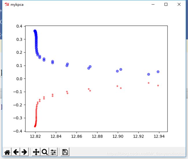
利用手写的kpca进行降维:
    def rbf_kernel_PCA_my(self, attributes, compents,gamma):
        m, n = attributes.shape
        dist = np.zeros((m, m))
        for i in range(m):
            dist[i] = np.sum(np.square(attributes[i] - attributes), axis=1).reshape(1, m)


        # 将成对距离转换成方阵。

        k =np.exp(-gamma * dist)

        #将内核矩阵中心化 具体用处还有点蒙蔽
        ln = np.ones((m,m))/n
        kp = k-ln.dot(k)-k.dot(ln)+ln.dot(k).dot(ln)
        lamda, V = np.linalg.eigh(kp)
        index = np.argsort(-lamda)[:compents]
        diag_lamda = np.sqrt(np.diag(-np.sort(-lamda)[:compents]))
        # 取出对应的特征向量矩阵
        V_selected = V[:, index]
        Z = V_selected.dot(diag_lamda)
        print np.sum(V_selected)
        return Z;
结果显示:
画图代码:“
plt.scatter(X[y == 0, 0], X[y == 0, 1], color='red', marker='^', alpha=0.5)
plt.scatter(X[y == 1, 0], X[y == 1, 1], color='blue', marker='o', alpha=0.5)

plt.tight_layout()
# plt.savefig('./figures/half_moon_1.png', dpi=300)
plt.show()
new1 = tool.rbf_kernel_PCA_my(attributes,2,0.5)
new2 = tool.rbf_kernel_PCA_sk(attributes,2,0.5)
plt.figure("mypca")
plt.scatter(new1[:,0],new1[:,1],c=iris.target)

plt.figure("sklearn-PCA")
plt.scatter(new2[:,0],new2[:,1],c=iris.target)
plt.show()
”
利用skearn中的kpac进行降维:
 def rbf_kernel_PCA_sk(self, attributes, compents, gamma):
        from sklearn.decomposition import PCA, KernelPCA
        kpca = KernelPCA(kernel="rbf", n_components=compents,gamma=gamma)
        x_kpca = kpca.fit_transform(attributes)
        return x_kpca;
