时域卷积与频域乘积
原文:http://www.ilovematlab.cn/thread-443872-1-1.html
Correlationconvolution相关 卷积
卷积定理:时域的卷积等于频域乘积
情况一,矩阵不拓展:
p=[0,-1,0;-1,4,-1;0,-1,0];%矩阵1
x=magic(5);%矩阵2
a=conv2(x,p,'same');%卷积结果
P=fft2(p,5,5);%矩阵1FFT
X=fft2(x);%矩阵2FFT
aa=X.*P;%频域乘积
r=ifft2(aa);%频域转换
a=
21 73 -35 2 36
66 -40 -5 5 13
-23 -10 0 10 49
13 -5 5 40 -40
16 24 61 -47 31
r =
5.0000 -10.0000 0 60.0000 -55.0000
10.0000 -5.0000 55.0000 -60.0000 0.0000
-10.0000 50.0000 -40.0000 -5.0000 5.0000
45.0000 -45.0000 -10.0000 0.0000 10.0000
-50.0000 10.0000 -5.0000 5.0000 40.0000
情况二,矩阵拓展:
p=[0,-1,0;-1,4,-1;0,-1,0];%矩阵1
x=magic(5);%矩阵2
a=conv2(x,p,'full');%卷积结果
P=fft2(p,7,7);%矩阵1FFT
X=fft2(x,7,7);%矩阵2FFT
aa=X.*P;%频域乘积
r=ifft2(aa);%频域转换
a=
0 -17 -24 -1 -8 -15 0
-17 21 73 -35 2 36 -15
-23 66 -40 -5 5 13 -16
-4 -23 -10 0 10 49 -22
-10 13 -5 5 40 -40 -3
-11 16 24 61 -47 31 -9
0 -11 -18 -25 -2 -9 0
r =
-0.0000 -17.0000 -24.0000 -1.0000 -8.0000 -15.0000 -0.0000
-17.0000 21.0000 73.0000 -35.0000 2.0000 36.0000 -15.0000
-23.0000 66.0000 -40.0000 -5.0000 5.0000 13.0000 -16.0000
-4.0000 -23.0000 -10.0000 -0.0000 10.0000 49.0000 -22.0000
-10.0000 13.0000 -5.0000 5.0000 40.0000 -40.0000 -3.0000
-11.0000 16.0000 24.0000 61.0000 -47.0000 31.0000 -9.0000
0.0000 -11.0000 -18.0000 -25.0000 -2.0000 -9.0000 -0.0000
在处理图像时,所用到的图像复原,都是在时域上做卷积,处理时都是将其转化到频域做乘积,然后再做傅里叶反变换。
但是函数在转化成频域时,做傅里叶变化并没有对矩阵扩展。。
例如图像I为[n,m]大小,掩膜P为[a,b].处理时是将P扩展到[n,m]大小,即fft2(P,a,b);
而不是将I和P都扩展到[n+a-1,m+b-1];
经验证,都扩展到[n+a-1,m+b-1]再做频域乘积,在经过傅里叶反变换得到的结果才和时域卷积的结果一致。
保持[n,m]大小得到的结果是不对的。
例如我上面写道的情况1和情况2,分别对应这两种情况。
掩膜:
C = conv2(A, B) performs the 2-D convolution of matrices A and B.
If [ma,na] = size(A), [mb,nb] = size(B), and [mc,nc] = size(C), then
mc = max([ma+mb-1,ma,mb]) and nc = max([na+nb-1,na,nb]).
C = conv2(H1, H2, A) first convolves each column of A with the vector
H1 and then convolves each row of the result with the vector H2. If
n1 = length(H1), n2 = length(H2), and [mc,nc] = size(C) then
mc = max([ma+n1-1,ma,n1]) and nc = max([na+n2-1,na,n2]).
conv2(H1, H2, A) is equivalent to conv2(H1(:)*H2(:).', A) up to
round-off.
C = conv2(..., SHAPE) returns a subsection of the 2-D
convolution with size specified by SHAPE:
'full' - (default) returns the full 2-D convolution,
'same' - returns the central part of the convolution
that is the same size as A.
'valid' - returns only those parts of the convolution
that are computed without the zero-padded edges.
size(C) = max([ma-max(0,mb-1),na-max(0,nb-1)],0).
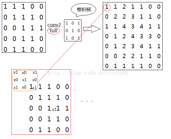
关于full, same以及valid三种参数的区别,如下面的实例所示:
full
same

valid
