非线性映射——核主成分分析
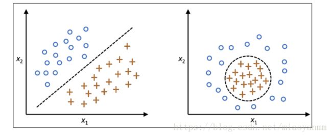
许多机器学习算法都假定输入数据是线性可分的。感知器为了保证其收敛性,甚至要求训练数据是完美线性可分的。然而,在现实世界中,大多数情况下我们面对的是非线性问题,针对此类问题,通过降维技术,如PCA和LDA等,将其转化为线性问题并不是最好的办法。
核函数与核技巧
通过将非线性可分问题映射到维度更高的特征空间,使其在新的特征空间上线性可分。为了将样本 x∈Rd x ∈ R d 转换到维度更高的 k 维子空间,定义如下非线性映射函数 ϕ ϕ :

我们可以将 ϕ ϕ 看做是一个函数,它能够对原始特征进行非线性映射,以将原始的 d 维数据集映射到更高的 k 维特征空间。例如:对于二维(d = 2)特征向量 x∈Rd x ∈ R d 来说,可用如下映射将其转换到三维空间:

换句话说,利用核PCA,可以通过非线性映射将数据转换到一个高维空间,然后在此高维空间中使用标准PCA将其映射到另外一个低维空间中,并通过线性分类器进行划分(前提条件,样本可根据输入空间的密度进行划分)。但是,这种方法的确定是带来高昂的计算成本,这也是为什么要使用核技巧的原因。通过使用核技巧,可以在原始特征空间中计算两个高维特种空间中向量的相似度。
在更深入了解使用核技巧解决计算成本高昂的问题之前,先回顾一下标准PCA方法。两个特征 k 和 j 之间协方差的计算公式如下:

由于在对特征做标准化处理后,其均值为0,所以上述公式可简化为:

由此可得出计算协方差矩阵 Σ Σ 的通用公式:

可以使用 ϕ ϕ 通过在原始特征空间上的非线性特征组合来替代样本间点积的计算:

为了求得此协方差矩阵的特征向量,也就是主成分,需要求解下述公式:
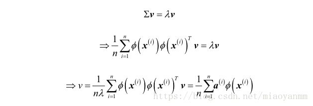
其中, λ λ 和 ν ν 分别为协方差矩阵 Σ Σ 的特征值和特征向量,这里 α α 可以通过提取核(相似)矩阵 K K 的特征向量来得到。
核矩阵的推导过程如下:
首先,使用矩阵符号来表示协方差矩阵,其中 ϕ(X) ϕ ( X ) 是一个 n * k维的矩阵:

现在,可以将特征向量的公式记为:

由于 Σν=λν Σ ν = λ ν ,可以得到:

两边同乘以 ϕ(X) ϕ ( X ) , 可得:

其中, K K 为相似(核)矩阵:
![]()
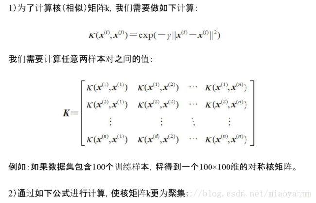
通过核函数 K K 以避免使用 ϕ ϕ 来精确计算样本集合 X X 中样本对之间的点积,这样就无需对特征向量进行精确的计算:

通过核 PCA ,能够得到已经映射到各成分的样本,而不像标准 PCA 方法那样去构建一个转换矩阵。简单地说,可以将核函数理解为:通过两个向量点积来度量向量间相似度的函数。常用的核函数有:


综合上述讨论,可以通过如下三个步骤来实现一个基于 RBF 核的 PCA :

核主成分分析实现
from scipy.spatial.distance import pdist, squareform
from scipy import exp
from scipy.linalg import eigh
import numpy as np

def rbf_kernel_pca(X, gamma, n_components):
    """
    RBF kernel PCA implementation.

    Parameters
    __________
    X: {Numpy ndarray}, shape = [n_samples, n_features]

    gamma: float
        Tuning parameters of the RBF kernel

    n_components: int
        Number of principal components to return

    Returns
    __________
    X_pc: {Numpy ndarray}, shape = [n_samples, k_features]
        Projected dataset

    """
    # Calculate pairwise squared Euclidean distances
    # in the MxN dimensional dataset.
    sq_dist = pdist(X, 'sqeuclidean')

    # Convert pairwise distances into a square matrix.
    mat_sq_dists = squareform(sq_dist)

    # Compute the symmetric kernel matrix.
    K = exp(-gamma * mat_sq_dists)

    # Center the kernel matrix.
    N = K.shape[0]
    one_n = np.ones((N, N)) / N
    K = K - one_n.dot(K) - K.dot(one_n) + one_n.dot(K).dot(one_n)

    # Obtaining eigenpairs from the centered kernel matrix
    # scipy.linalg.eigh returns them in ascending order
    eigvals, eigvecs = eigh(K)

    # Collect the top K eigenvectors (projected samples)
    X_pc = np.column_stack((eigvecs[:, -i] for i in range(1, n_components + 1)))

    return X_pc
案例1:分离半月形数据
首先创建一个保护100个样本点的二维数据集,以两个半月形状表示:
from sklearn.datasets import make_moons
X, y = make_moons(n_samples=100, random_state=123)

import matplotlib.pyplot as plt
plt.scatter(X[y == 0, 0], X[y == 0, 1], color='red', marker='^', alpha=0.5)
plt.scatter(X[y == 1, 0], X[y == 1, 1], color='blue', marker='o', alpha=0.5)
plt.show()
显然,这两个半月形不是线性可分的,而我们的目标是通过核 PCA 将这两个半月形数据展开,使得数据集成为适用于某一线性分类器的输入数据。
首先,通过标准 PCA 将数据映射到主成分上,并观察其形状:
from sklearn.decomposition import PCA
scikit_pca = PCA(n_components=2)
X_spca = scikit_pca.fit_transform(X)
fig, ax = plt.subplots(nrows=1, ncols=2, figsize=(7, 3))
ax[0].scatter(X_spca[y == 0, 0], X_spca[y == 0, 1], color='red', marker='^', alpha=0.5)
ax[0].scatter(X_spca[y == 1, 0], X_spca[y == 1, 1], color='blue', marker='o', alpha=0.5)
ax[1].scatter(X_spca[y == 0, 0], np.zeros((50, 1)) + 0.02, color='red', marker='^', alpha=0.5)
ax[1].scatter(X_spca[y == 1, 0], np.zeros((50, 1)) - 0.02, color='blue', marker='o', alpha=0.5)
ax[0].set_xlabel('PC1')
ax[0].set_ylabel('PC2')
ax[1].set_ylim([-1, 1])
ax[1].set_yticks([])
ax[1].set_xlabel('PC1')
plt.show()
很明显,经过标准 PCA 的转换后,线性分类器未能很好地发挥其作用。
使用核 PCA 函数:rbf_kernel_pca
from matplotlib.ticker import FormatStrFormatter
X_kpca = rbf_kernel_pca(X, gamma=15, n_components=2)
fig, ax = plt.subplots(nrows=1, ncols=2, figsize=(7, 3))
ax[0].scatter(X_kpca[y == 0, 0], X_kpca[y == 0, 1], color='red', marker='^', alpha=0.5)
ax[0].scatter(X_kpca[y == 1, 0], X_kpca[y == 1, 1], color='blue', marker='o', alpha=0.5)
ax[1].scatter(X_kpca[y == 0, 0], np.zeros((50, 1)) + 0.02, color='red', marker='^', alpha=0.5)
ax[1].scatter(X_kpca[y == 1, 0], np.zeros((50, 1)) - 0.02, color='blue', marker='o', alpha=0.5)
ax[0].set_xlabel('PC1')
ax[0].set_ylabel('PC2')
ax[1].set_ylim([-1, 1])
ax[1].set_yticks([])
ax[1].set_xlabel('PC1')
ax[0].xaxis.set_major_formatter(FormatStrFormatter('%0.1f'))
ax[1].xaxis.set_major_formatter(FormatStrFormatter('%0.1f'))
plt.show()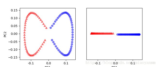
可以看到,两个类别(圆形和三角形)此时是线性可分的,这使得转换后的数据适合作为线性分类器的训练数据集。
案例2:分离同心圆数据
from sklearn.datasets import make_circles
X, y = make_circles(n_samples=1000, random_state=123, noise=0.1, factor=0.2)
plt.scatter(X[y == 0, 0], X[y == 0, 1], color='red', marker='^', alpha=0.5)
plt.scatter(X[y == 1, 0], X[y == 1, 1], color='blue', marker='o', alpha=0.5)
plt.show()
首先使用标准 PCA 方法:
scikit_pca = PCA(n_components=2)
X_spca = scikit_pca.fit_transform(X)
fig, ax = plt.subplots(nrows=1, ncols=2, figsize=(7, 3))
ax[0].scatter(X_spca[y == 0, 0], X_spca[y == 0, 1], color='red', marker='^', alpha=0.5)
ax[0].scatter(X_spca[y == 1, 0], X_spca[y == 1, 1], color='blue', marker='o', alpha=0.5)
ax[1].scatter(X_spca[y == 0, 0], np.zeros((500, 1)) + 0.02, color='red', marker='^', alpha=0.5)
ax[1].scatter(X_spca[y == 1, 0], np.zeros((500, 1)) - 0.02, color='blue', marker='o', alpha=0.5)
ax[0].set_xlabel('PC1')
ax[0].set_ylabel('PC2')
ax[1].set_ylim([-1, 1])
ax[1].set_yticks([])
ax[1].set_xlabel('PC1')
plt.show()
再一次发现,通过标准 PCA 无法得到适合于线性分类器的训练数据。
X_kpca = rbf_kernel_pca(X, gamma=15, n_components=2)
fig, ax = plt.subplots(nrows=1, ncols=2, figsize=(7, 3))
ax[0].scatter(X_kpca[y == 0, 0], X_kpca[y == 0, 1], color='red', marker='^', alpha=0.5)
ax[0].scatter(X_kpca[y == 1, 0], X_kpca[y == 1, 1], color='blue', marker='o', alpha=0.5)
ax[1].scatter(X_kpca[y == 0, 0], np.zeros((500, 1)) + 0.02, color='red', marker='^', alpha=0.5)
ax[1].scatter(X_kpca[y == 1, 0], np.zeros((500, 1)) - 0.02, color='blue', marker='o', alpha=0.5)
ax[0].set_xlabel('PC1')
ax[0].set_ylabel('PC2')
ax[1].set_ylim([-1, 1])
ax[1].set_yticks([])
ax[1].set_xlabel('PC1')
ax[0].xaxis.set_major_formatter(FormatStrFormatter('%0.1f'))
ax[1].xaxis.set_major_formatter(FormatStrFormatter('%0.1f'))
plt.show()
基于 RBF 的核 PCA 再一次将数据映射到了一个新的子空间中,使得两个类别变得线性可分。
映射新的数据点
我们从聚集核矩阵中得到了特征向量 α α ,这意味着样本已经映射到了主成分轴上。由此,如果我们希望将新的样本 x⋅ x ⋅ 映射到主成分轴,需要进行如下计算:

幸运的是,我们可以使用核技巧,这样就无需精确计算映射 ϕ(x⋅)Tν ϕ ( x ⋅ ) T ν 。需要注意的是,与标准 PCA 相比,核 PCA 是一种基于内存的方法,这意味着每次映射新的样本前,必须再次使用原始训练数据。

在完成新样本与训练数据集内样本间相似度的计算后,还需通过特征向量对应的特征值来对其进行归一化处理。可以通过修改前面实现过的 rbf_kernel_pca 函数来让其返回核矩阵的特征值:
from scipy.spatial.distance import pdist, squareform
from scipy import exp
from scipy.linalg import eigh
import numpy as np

def rbf_kernel_pca(X, gamma, n_components):
    """
    RBF kernel PCA implementation.

    Parameters
    __________
    X: {Numpy ndarray}, shape = [n_samples, n_features]

    gamma: float
        Tuning parameters of the RBF kernel

    n_components: int
        Number of principal components to return

    Returns
    __________
    X_pc: {Numpy ndarray}, shape = [n_samples, k_features]
        Projected dataset

    """
    # Calculate pairwise squared Euclidean distances
    # in the MxN dimensional dataset.
    sq_dist = pdist(X, 'sqeuclidean')

    # Convert pairwise distances into a square matrix.
    mat_sq_dists = squareform(sq_dist)

    # Compute the symmetric kernel matrix.
    K = exp(-gamma * mat_sq_dists)

    # Center the kernel matrix.
    N = K.shape[0]
    one_n = np.ones((N, N)) / N
    K = K - one_n.dot(K) - K.dot(one_n) + one_n.dot(K).dot(one_n)

    # Obtaining eigenpairs from the centered kernel matrix
    # scipy.linalg.eigh returns them in ascending order
    eigvals, eigvecs = eigh(K)

    # Collect the top K eigenvectors (projected samples)
    alphas = np.column_stack((eigvecs[:, -i] for i in range(1, n_components + 1)))

    # Collect the corresponding eigenvalues
    lambdas  = [eigvals[-i] for i in range(1, n_components + 1)]

    return alphas, lambdas
至此,可以创建一个新的半月形数据集,并使用更新过的 RBF 核 PCA 实现将其映射到一个一维子空间上:
X, y = make_moons(n_samples=100, random_state=123)
alphas, lambdas = rbf_kernel_pca(X, gamma=15, n_components=1)
x_new = X[25]
x_proj = alphas[25]
def project_x(x_new, X, gamma, alphas, lambdas):
    pair_dist = np.array([np.sum((x_new - row) ** 2) for row in X])
    k = np.exp(-gamma * pair_dist)
    return k.dot(alphas / lambdas)

x_reproj = project_x(x_new, X, gamma=15, alphas=alphas, lambdas=lambdas)

plt.scatter(alphas[y == 0, 0], np.zeros((50)), color='red', marker='^', alpha=0.5)
plt.scatter(alphas[y == 1, 0], np.zeros((50)), color='blue', marker='o', alpha=0.5)
plt.scatter(x_proj, 0, color='black', label='original projection of point X[25]',
    marker='^', s=100)
plt.scatter(x_reproj, 0, color='green', label='remapped point X[25]',
    marker='x', s=500)
plt.legend(scatterpoints=1)
plt.show()

scikit-learn中的核主成分分析
from sklearn.decomposition import KernelPCA
from sklearn.datasets import make_moons
import  matplotlib.pyplot as plt
X, y = make_moons(n_samples=100, random_state=123)
scikit_kpca = KernelPCA(n_components=2, kernel='rbf', gamma=15)
X_skernpca = scikit_kpca.fit_transform(X)
plt.scatter(X_skernpca[y == 0, 0], X_skernpca[y == 0, 1], color='red', marker='^', alpha=0.5)
plt.scatter(X_skernpca[y == 1, 0], X_skernpca[y == 1, 1], color='blue', marker='o', alpha=0.5)
plt.xlabel('PC1')
plt.ylabel('PC2')
plt.show()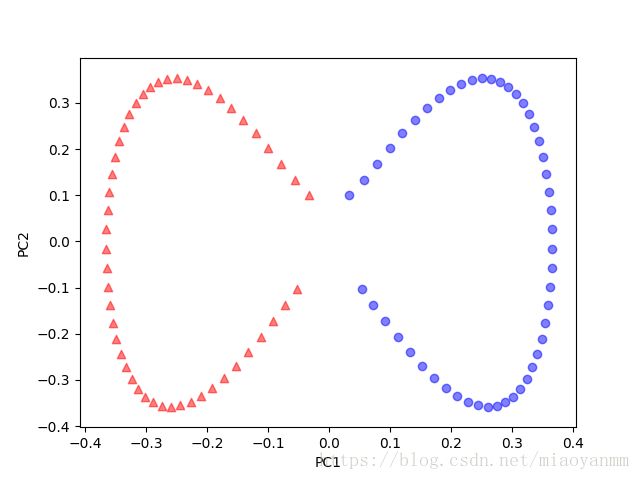
从结果图像中可以得知,通过scikit-learn中的KernelPCA得到的结果与我们自己实现的结果一致。
参考文献:
Python-Machine-Learning/Chapter 5: Compressing Data via Dimensionality Reduction