吴恩达逻辑回归---仿线性回归写的梯度下降，未引入优化算法

导入包

import numpy as np
import pandas as pd
import matplotlib.pyplot as plt

导入数据

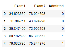
path=“ex2data1.txt”
data=pd.read_csv(path,header=None,names=[‘Exam1’,‘Exam2’,‘Admitted’])
data.head()


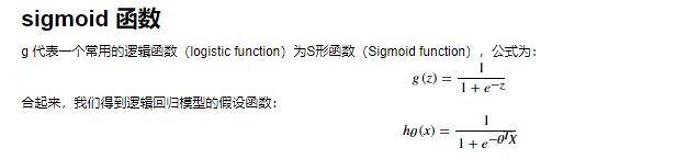
def sigmoid(z):

return 1/(1+np.exp(-z))

data.insert(0,‘Ones’,1)
data.head()

处理数据

cols=data.shape[1]
X=data.iloc[:,0:cols-1]
y=data.iloc[:,cols-1:cols]
X=np.matrix(X.values)
y=np.matrix(y.values)
theta=np.matrix(np.array([0,0,0]))
X.shape,y.shape,theta.shape



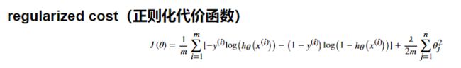
def cost(theta, X, y, learningRate):

first = np.multiply(-y, np.log(sigmoid(X * theta.T)))
second = np.multiply((1 - y), np.log(1 - sigmoid(X * theta.T)))
reg = (learningRate / (2 * len(X))) * np.sum(np.power(theta[:,1:theta.shape[1]], 2))
return np.sum(first - second) / (len(X))+ reg

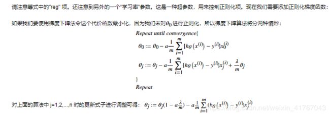
学习率不易过高是因为在实际计算中发现过高会得到区间最优解

alpha=0.0005
cost(theta, X, y,alpha)

def gradientDescent(X,y,theta,alpha,iters):

temp=np.matrix(np.zeros(theta.shape))

parameters=int(theta.ravel().shape[1])

for i in range(iters):
    error = sigmoid(X * theta.T) - y
    for j in range(parameters):
        term=np.multiply(error,X[:,j])
        if (j == 0):
            temp[0,j]=theta[0,j]-((alpha/len(X))*np.sum(term))
        else:
            temp[0,j]=theta[0,j]-((alpha/len(X))*np.sum(term)) + ((alpha / len(X)) * theta[:,j])
    theta=temp
    
return theta

iters=1000000
g=gradientDescent(X,y,theta,alpha,iters)

cost(g, X, y,alpha)

正确率

def predict(theta,X):

probability=sigmoid(X*theta.T)
return [1 if x>=0.5 else 0 for x in probability]

predictions = predict(g, X)
correct = [1 if ((a == 1 and b == 1) or (a == 0 and b == 0)) else 0 for (a, b) in zip(predictions, y)]
accuracy = (sum(map(int, correct)) % len(correct))
print (‘accuracy = {0}%’.format(accuracy))

使用这个方法可以看出正确率要比优化参数算法的正确率高，缺点是迭代次数太多