cs231n-assignment1的笔记

在看完cs231n前面几章的内容后，准备做一下assignment1，然后怕之后忘记，所以写博文记录一下......

由于我是个low逼程序员，平时能用Windows就绝不用linux，所以在这次作业时使用虚拟机完成了作业，装好ubuntu16.04之后，配好环境，使用jupyter notebook查看相应的要求

Q1: k-Nearest Neighbor classifier

由于我对matplotlib并不是特别的熟悉，这里面学到的第一个点就是画图像的预览图，plt.imshow(a)中a的格式要求是width*height*depth,数据类型是无符号整型(uint8),代码如下：

classes = ['plane', 'car', 'bird', 'cat', 'deer', 'dog', 'frog', 'horse', 'ship', 'truck']
num_classes = len(classes)
samples_per_class = 7  # 每种类型采7个样
for y, cls in enumerate(classes): #enumerate(list)会返回index以及value
    idxs = np.flatnonzero(y_train == y)  # 取出与y标签相同的数据的索引，numpy中的flatnonzero就是取出非零的索引
    idxs = np.random.choice(idxs, samples_per_class, replace=False)  # 从中取样（7个）
        for i, idx in enumerate(idxs):
            plt_idx = i * num_classes + y + 1
            plt.subplot(samples_per_class, num_classes, plt_idx) # 参数1代表行数、参数2代表列数、参数3代表第几个图，之所以每次都需要输入第1、2个参数，这两个参数是可变的
            plt.imshow(X_train[idx].astype('uint8')) # 在上一条指令指定好绘制区域后，进行特定图像显示
            plt.axis('off')
            if i == 0:
		plt.title(cls) # 仅在第一个图上面显示title
plt.show()

然后就开始实现cs231n/classifiers/k_nearest_neighbor.py中的compute_distances_two_loops函数，其实也就是一行代码dists[i, j] = np.sqrt(np.sum((X[i]-self.X_train[j])**2))

这里的知识点是计算两个vector的L2距离，所以可以简单粗暴的直接求解。

然后画出dist的分布图之后有一个问题，问白横线和白竖线分别是怎么造成的，白横线代表某一个测试样本与训练样本的距离都比较大，白竖线表示某个训练样本与测试样本的距离较大

然后要实现predict_labels

首先利用距离矩阵dists找出k个与测试样本i最近的训练样本的label，利用np.argsort可以找出dists中最小的k个值的index，然后利用index取出对应的label即可得到closest_y

closest_y = self.y_train[np.argsort(dists[i])[0:k]]

在得到closest_y之后，找到k近邻中label出现次数最多的label返回，利用np.bincount(y)可以统计y中元素出现的次数，并且返回出现次数，bincount的返回值a的每一项对应一个值出现次数，例如a[0]代表的是y中0出现次数，a[1]代表y中1出现次数......然后利用argmax求出出现次数最多的元素，返回即可：

y_pred[i] = np.argmax(np.bincount(closest_y))

之后是实现一层循环求解以及不用循环求解，这里其实也就是矩阵的操作

一层循环中循环次数为测试样例的个数，所以在循环体中要实现vector和matrix的距离求解，与上面的方法是相似的

不用循环的方法则有一点trick，首先将L2距离公式展开，然后分别求平方项以及叉积。

dists[i, :] = np.sqrt(np.sum(((self.X_train - X[i])**2), axis = 1))

dists += np.sum(self.X_train**2, axis=1).reshape(1, num_train) # 这里其实利用了broadcast
dists += np.sum(X**2, axis=1).reshape(num_test, 1)
dists -= 2 * np.dot(X, self.X_train.T) # np.dot(a,b)可以对两个矩阵求乘积，要求a的第二维与b的第一维长度一致
dists = np.sqrt(dists)

后面是交叉验证部分，也就是抽出一部分数据作为测试集，一部分为验证集，其余为训练集，采用的是5折交叉验证法，首先将训练数据进行划分，按照作业提示，使用np.array_split将数据划分为5块，如下：

y_train_ = y_train.reshape(-1, 1)
X_train_folds = np.array_split(X_train, num_folds)
y_train_folds = np.array_split(y_train, num_folds)

然后先对k_to_accuracies赋初始值[]，利用两层循环进行交叉验证，外层循环为folds数，内层循环为不同的k值，这里比较简单，仅写出解决的代码

for k_ in k_choices:
    k_to_accuracies.setdefault(k_, [])
for i in range(num_folds):
    classifier = KNearestNeighbor()
    X_val_train = np.vstack(X_train_folds[0:i] + X_train_folds[i+1:])
    y_val_train = np.vstack(y_train_folds[0:i] + y_train_folds[i+1:])
    y_val_train = y_val_train[:,0]
    classifier.train(X_val_train, y_val_train)
    for k_ in k_choices:
        y_val_pred = classifier.predict(X_train_folds[i], k=k_)
        num_correct = np.sum(y_val_pred == y_train_folds[i][:,0])
        accuracy = float(num_correct) / len(y_val_pred)
        k_to_accuracies[k_] = k_to_accuracies[k_] + [accuracy]

Q2: Training a Support Vector Machine

前3步与前面knn的步骤差不多，然后第四步开始将数据分为训练集、验证集和测试集，50000个训练集中49000作为训练集，1000作为验证集。测试集只选取10000个测试样本中的前1000个。

然后从这49000个训练集中选取出500个开发集，用于调参，使用的函数为:np.random.choice(num_training, num_dev, replace=False)

第六步中求了这49000个训练集的均值并且显示，然后第七步中对所有数据进行了中心化（中心化是减去均值，标准化是减去均值后除以标准差，这个与统计学概念类似），对训练集、验证集、开发集以及测试集均减去前述49000个训练集的均值。

然后在每一条数据记录后面加上1，以便于只关注W，而不用关注b(也即是f(x, W) = Wx + b，x=(x1, x2, x3...xn)将x增加1，即x=(x1, x2, x3...xn, 1)，然后f(x, W) = Wx, 其中W的最后一项即原式中的b，这个在cs229中有讲过)

后面正式开始svm分类器

svm_loss_naive

在linear_svm.py中第一种实现方式是比较naive的方式，计算loss时利用两层循环进行，对于每一个训练集，利用其乘以W之后，得到其对每个类的得分score以及正确标签的得分correct_class_score, 然后内层循环对每个类，分别计算max(0, score-correct_class_score+1), loss值为输入的所有X的loss之和的均值，然后加上一个L2正则项以防止W过于复杂，即total_loss = avg_loss + lambda *  sum(W*W), 后面是我们要实现求dW, 也即求梯度，后面的代码会进行检查，比较numerical和analytic两种方式的差别，而我们要实现的就是analytical方式

根据cs231n的notes点击打开链接, Loss function对w的偏导，公式如下所示：

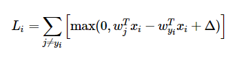
由于wyi在每一个max(0, wj * xi - wyi * xi + delta)中都出现了，所以求dW时每次都要加上对wyi的偏导，即在原代码中内层循环加上：

dW[:, j] += X[i].T
dW[:, y[i]] -= X[i].T

后面的偏导就看loss的变化，所以svm_loss_naive函数最后实现如下所示：

def svm_loss_naive(W, X, y, reg):
  """
  Structured SVM loss function, naive implementation (with loops).

  Inputs have dimension D, there are C classes, and we operate on minibatches
  of N examples.

  Inputs:
  - W: A numpy array of shape (D, C) containing weights.
  - X: A numpy array of shape (N, D) containing a minibatch of data.
  - y: A numpy array of shape (N,) containing training labels; y[i] = c means
    that X[i] has label c, where 0 <= c < C.
  - reg: (float) regularization strength

  Returns a tuple of:
  - loss as single float
  - gradient with respect to weights W; an array of same shape as W
  """
  dW = np.zeros(W.shape) # initialize the gradient as zero

  # compute the loss and the gradient
  num_classes = W.shape[1]
  num_train = X.shape[0]
  loss = 0.0
  for i in xrange(num_train):
    scores = X[i].dot(W)
    correct_class_score = scores[y[i]]
    for j in xrange(num_classes):
      if j == y[i]:
        continue
      margin = scores[j] - correct_class_score + 1 # note delta = 1
      if margin > 0:
        loss += margin
        dW[:, j] += X[i].T
        dW[:, y[i]] -= X[i].T # 在loss公式的每一项中均出现,所以每次都要加上这一项

      # Right now the loss is a sum over all training examples, but we want it
  # to be an average instead so we divide by num_train.
  loss /= num_train
  dW /= num_train
  # Add regularization to the loss.
  loss += reg * np.sum(W * W)
  dW += 2 * reg * W

  #############################################################################
  # TODO:                                                                     #
  # Compute the gradient of the loss function and store it dW.                #
  # Rather that first computing the loss and then computing the derivative,   #
  # it may be simpler to compute the derivative at the same time that the     #
  # loss is being computed. As a result you may need to modify some of the    #
  # code above to compute the gradient.                                       #
  #############################################################################


  return loss, dW

Inline Question1问的是什么时候两种梯度计算方式结果不同，很简单，对于分段函数，一般边界点的导数是不同的

接下来是使用vector操作实现loss和dW的计算，首先是loss，这个比较简单，利用矩阵的基础知识就可以写出相应代码：

num_train = X.shape[0]
y_f = np.dot(X, W)
y_c = y_f[range(num_train), list(y)].reshape(-1, 1)
margins = np.maximum(y_f - y_c + 1, 0)# shape [N, C]
margins[range(num_train), list(y)] = 0
loss = np.sum(margins) / num_train + reg * np.sum(W * W)

其实也就是循环实现方式的向量化

然后是实现dW的计算，根据上面循环方式的实现可知，对于一个sample而言，在margin[i]大于0时 (00)就加上1，然后在y[i]列减去1，然后直接用data.T乘以mask，就能得到dW的值，根据前面得到的margins，其大于0的部分便是结果，所以mask定义为margins>0的部分为1，然后对于每个y[i]列（即每个样本的真实标记），将mask每行的和的负数赋值给sample真实标记所在位置，其余步骤与loss处理一致，代码如下所示：

mask = margins
mask[margins > 0] = 1
mask[range(num_train), list(y)] = -np.sum(mask, axis=1)

dW = (X.T).dot(mask)
dW = dW/num_train + 2 * reg * W

后面是SGD，首先实现train函数，sample的方式也就是一般机器学习里的技巧，利用np.random.choice()生成index，然后取X，y中的对应项，而更新W的方式更加简单，梯度下降，W = W - lr * dW, 代码如下：

index = np.random.choice(range(X.shape[0]), batch_size, replace=True)
X_batch = X[index]
y_batch = y[index]

self.W -= learning_rate * grad

接下来是实现预测函数predict，这个较简单，一行代码搞定：

y_pred = np.argmax(X.dot(self.W), axis=1)

接下来是实现寻找最优超参的过程：

for reg in regularization_strengths:
    for lr in learning_rates:
        svm = LinearSVM()
        loss_hist = svm.train(X_train, y_train, lr, reg, num_iters=1500)
        y_train_pred = svm.predict(X_train)
        train_accuracy = np.mean(y_train == y_train_pred)
        y_val_pred = svm.predict(X_val)
        val_accuracy = np.mean(y_val == y_val_pred)
        if val_accuracy > best_val:
            best_val = val_accuracy
            best_svm = svm
        results[(lr, reg)] = train_accuracy, val_accuracy

Q3: Implement a Softmax classifier

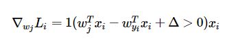
实现softmax, 首先是naive方式，即for循环实现，根据notes点击打开链接中的提示，计算exp的值有时候会变得十分之大。例如exp(500)之类的值，所以一般利用减去最大值使得其余的值均小于0，此时exp(x)的值仅在(0, 1]之间，证明公式如下所示：

一般利用计算

而求dW则就是简单的求导法则了，自己用笔推算了一下，如下：

再与之前一样，加上正则项，完成，所以softmax_loss_naive函数的具体实现如下：

num_train = X.shape[0]
num_classes = W.shape[1]
for i in range(num_train):
  scores = X[i].dot(W)
  adjust_scores = scores - np.max(scores)
  loss_t = -np.log(np.exp(adjust_scores[y[i]]) / np.sum(np.exp(adjust_scores)))
  loss += loss_t
  for j in range(num_classes):
    prob = np.exp(adjust_scores[j]) / np.sum(np.exp(adjust_scores))
    if j == y[i]:
      dW[:, j] += (-1 + prob) * X[i]
    else:
      dW[:, j] += prob * X[i]

loss = loss / num_train
dW = dW / num_train
loss += reg * np.sum(W * W)
dW += 2 * reg * W

然后测试中为何要使loss接近-log(0.1)，这是因为我们的W是随机生成的，所以其对于每个class得到的结果在概率上应该差距不大，总class为10，则其正确的概率就是0.1

接下来是实现向量化的softmax，对于loss的求解较简单不再赘述，dW的求解与前述的求导是一致的，与Q2中的mask类似，根据前面naive的实现方式可知，在j==y[i]时需要-1,so 代码如下：

num_train = X.shape[0]
scores = X.dot(W)
adjust_scores = np.exp(scores - np.max(scores, axis=1).reshape(-1, 1))
sum_scores = np.sum(adjust_scores, axis=1).reshape(-1, 1)
class_prob = adjust_scores / sum_scores  # shape [N, C]
prob = class_prob[range(num_train), list(y)]
total_loss = -np.log(prob)
loss = np.sum(total_loss) / num_train + reg * np.sum(W * W)

class_prob[range(num_train), list(y)] -= 1
dW = (X.T).dot(class_prob)
dW = dW / num_train + 2 * reg * W

其中class_prob计算了所有的exp(fj)/sum(exp(f))......

接下来又是寻找最优超参的过程，与Q2的类似，不再说明。。。

for lr in learning_rates:
  for reg in regularization_strengths:
    softmax = Softmax()
    softmax.train(X_train, y_train, lr, reg, num_iters=3000)
    y_train_pred = softmax.predict(X_train)
    train_accuracy = np.mean(y_train == y_train_pred)
    y_val_pred = softmax.predict(X_val)
    val_accuracy = np.mean(y_val == y_val_pred)
    if val_accuracy > best_val:
      best_val = val_accuracy
      best_softmax = softmax
    results[(lr, reg)] = train_accuracy, val_accuracy

后面有一个可视化W的方法，虽然不是作业，但比较有意思，对于W，其shape是D * C，其中D是与输入X(图片)有关，C是类别数，然后对于W中的元素，归一化之后乘以255，得到相应的像素值，代码如下（来自cs231n-assignment1-softmax.ipynb）：

# Visualize the learned weights for each class
w = best_softmax.W[:-1, :]  # strip out the bias
print(w.shape)
w = w.reshape(32, 32, 3, 10)

w_min, w_max = np.min(w), np.max(w)

classes = ['plane', 'car', 'bird', 'cat', 'deer', 'dog', 'frog', 'horse', 'ship', 'truck']
for i in range(10):
  plt.subplot(2, 5, i + 1)

  # Rescale the weights to be between 0 and 255
  wimg = 255.0 * (w[:, :, :, i].squeeze() - w_min) / (w_max - w_min)
  plt.imshow(wimg.astype('uint8'))
  plt.axis('off')
  plt.title(classes[i])

Q4: Two-Layer Neural Network 

这里要实现两层神经网络，首先是loss函数中的scores的计算，根据lecture4的slides可以得知，多层神经网络的score函数如下所示：

根据公式写出scores的计算表达式：

h1 = np.maximum(0, (X.dot(W1) + b1))
scores = h1.dot(W2) + b2

然后实现loss, 前向传播过程，同时也需要加入正则项（题中使用L2正则项）,loss函数为Softmax classifier loss

adjust_scores = np.exp(scores - np.max(scores, axis=1).reshape(-1, 1)) # [N, C]
sum_scores = np.sum(adjust_scores, axis=1).reshape(-1, 1) # [N, 1]
class_prob = adjust_scores / sum_scores   # [N, C]
prob = class_prob[range(N), list(y)]  # [N, 1]
total_loss = -np.log(prob)  # [N, 1]
loss = np.sum(total_loss) / N + reg * (np.sum(W1 * W1) + np.sum(W2 * W2))

接下来是求gradients, 这个看起来无从下手，其实与之前Q3 的softmax是类似的，但我做Q3时还没看过Lecture4和5，所以直接推导公式，感觉很抽象不容易理解，看了lecture4点击打开链接的后向传播求梯度后就简单很多了。

求dW2和db2较简单，与之前softmax一致：

dscores = class_prob
dscores[range(N), list(y)] -= 1
dscores /= N
grads['W2'] = (h1.T).dot(dscores)
grads['b2'] = np.sum(dscores, axis=0)

根据scores = h1.dot(W2) + b2可知，dh1 = dscores.dot(W2.T)，由此可知：

dh1 = dscores.dot(W2.T)
dh1_raw = dh1 * (h1>0)
grads['W1'] = X.T.dot(dh1_raw) + 2 * reg * W1
grads['b1'] = np.sum(dh1_raw, axis=0)

接下来写train函数，第一部分与之前的一致，也就是随机采样：

index = np.random.choice(num_train, batch_size, replace=True)
X_batch = X[index]
y_batch = y[index]

更新参数：

self.params['W2'] -= learning_rate * grads['W2']
self.params['b2'] -= learning_rate * grads['b2']
self.params['W1'] -= learning_rate * grads['W1']
self.params['b1'] -= learning_rate * grads['b1']

最后是predict函数：

W1, b1 = self.params['W1'], self.params['b1']
W2, b2 = self.params['W2'], self.params['b2']
h1 = np.maximum(0, (X.dot(W1) + b1))
scores = h1.dot(W2) + b2
y_pred = np.argmax(scores, axis=1)

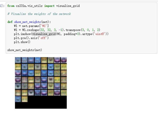
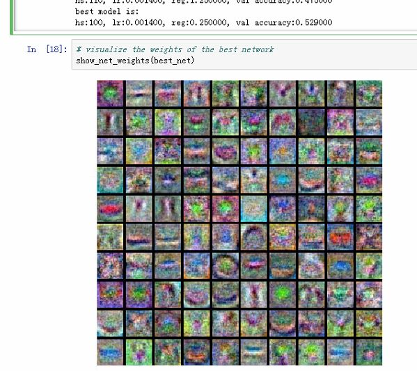
在debug the training中演示了如何debug,主要通过做出loss的图以及分类准确率，比较有意思的是将W1的图做出来了，可以发现W1中模糊可见一些汽车的影子，说明分类效果并不好：

接下来是寻找最优参数的过程：

best_val_acc = 0
best_lr = 0
best_hs = 0
best_reg = 0

learning_rates_base = 0.001
learning_rates_step = 0.0001
hidden_size_base = 60
hidden_size_step = 10
reg_base = 0.25
reg_step = 0.25

for hs_count in range(5):
    for lr_count in range(5):
        for reg_count in range(5):
            hs = hidden_size_base + hs_count * hidden_size_step
            lr = learning_rates_base + lr_count * learning_rates_step
            reg = reg_base + reg_count * reg_step
            net = TwoLayerNet(input_size, hs, num_classes)
            results = net.train(X_train, y_train, X_val, y_val,
                                num_iters=2000, batch_size=200,
                                learning_rate=lr, learning_rate_decay=0.95,
                                reg=reg, verbose=False)
            val_acc = np.mean(net.predict(X_val) == y_val)
            print("hs:%d, lr:%f, reg:%f, val accuracy:%f"%(hs, lr, reg, val_acc))
            if val_acc > best_val_acc:
                best_val_acc = val_acc
                best_net = net
                best_hs = hs
                best_lr = lr
                best_reg = reg
print("best model is:")
print("hs:%d, lr:%f, reg:%f, val accuracy:%f"%(best_hs, best_lr, best_reg, best_val_acc))

这个区间可以自己设置，我在hs  = 100, lr = 0.0014, reg = 0.25时取到最优结果，验证集准确率为52.9%。w1的图如下所示：

Q5: Higher Level Representations: Image Features

前面的作业是让神经网络训练寻找特征，但是通过对前面W1进行查看，发现其寻找到的特征并不是很理想，而这个作业则是通过改进特征提取过程来改进效果。

首先来看看features.py中的各个函数

extract_features函数就是应用各个feature functions, 然后组合而成新的特征向量，其中每个feature function应该返回一个一维向量，然后多个feature functions返回值组合形成新的特征向量。

rgb2gray就是将rgb图值转换为灰度图，这里直接使用公式：Gray = R*0.299 + G*0.587 + B*0.114

hog_feature则是提取方向梯度直方图

color_histogram_hsv利用hsv颜色模式计算颜色直方图

然后运行Extract Features中的代码时发现会提示错误：

slice indices must be integers or None or have an __index__ method

问题定位在features.py的121行，发现应该是python2和python3对除法的操作不一致所致，而slice操作需要的是一个整数，由于作业使用的环境应该是python2，而我使用的是python3，所以将该行代码改为整除的形式：

orientation_histogram[:,:,i] = uniform_filter(temp_mag, size=(cx, cy))[cx//2::cx, cy//2::cy].T

然后就正常了，接下来利用抽取的feature训练SVM分类，这个过程与之前的寻找最优参数的过程类似

for rs in regularization_strengths:
    for lr in learning_rates:
        svm = LinearSVM()
        svm.train(X_train_feats, y_train, lr, rs, num_iters=3000)
        y_train_pred = svm.predict(X_train_feats)
        train_accuracy = np.mean(y_train == y_train_pred)
        y_val_pred = svm.predict(X_val_feats)
        val_accuracy = np.mean(y_val == y_val_pred)
        if val_accuracy > best_val:
            best_val = val_accuracy
            best_svm = svm           
        results[(lr,rs)] = train_accuracy, val_accuracy

神经网络的与上类似，主要是调参过程，然而并没有找到合适的参数。。。

best_val_acc = 0
best_lr = 0
best_hs = 0
best_reg = 0

learning_rates_base = 0.01
learning_rates_step = 0.01
reg_base = 0.25
reg_step = 0.25

for lr_count in range(5):
    for reg_count in range(5):
        lr = learning_rates_base + lr_count * learning_rates_step
        reg = reg_base + reg_count * reg_step
        net = TwoLayerNet(input_dim, hidden_dim, num_classes)
        result = net.train(X_train_feats, y_train, X_val_feats, y_val,
                           num_iters=2000, batch_size=200,
                           learning_rate=lr, learning_rate_decay=0.95,
                           reg=reg, verbose=False)
        val_acc = np.mean(net.predict(X_val_feats) == y_val)
        print("hs:%d, lr:%f, reg:%f, val accuracy:%f"%(hs, lr, reg, val_acc))
        if val_acc > best_val_acc:
            best_val_acc = val_acc
            best_net = net
            best_lr = lr
            best_reg = reg
print("best model is:")
print("hs:%d, lr:%f, reg:%f, val accuracy:%f"%(best_hs, best_lr, best_reg, best_val_acc))

Q6: Cool Bonus: Do something extra! 

待填坑......