时间序列之模型优化
1、差分.diff(1)
一阶差分:
pd['diff_1'] = pd['row'].diff(1) #对列数据做差分
2、ACF和PACF的绘制
importstatsmodels.api assm

def tsplot(y, lags=None, title='', figsize=(14, 8)):

    fig = plt.figure(figsize=figsize)
    layout = (2, 2)
    ts_ax   = plt.subplot2grid(layout, (0, 0))
    hist_ax = plt.subplot2grid(layout, (0, 1))
    acf_ax  = plt.subplot2grid(layout, (1, 0))
    pacf_ax = plt.subplot2grid(layout, (1, 1))

    y.plot(ax=ts_ax)
    ts_ax.set_title(title)
    y.plot(ax=hist_ax, kind='hist', bins=25)

    hist_ax.set_title('Histogram')

    smt.graphics.plot_acf(y, lags=lags, ax=acf_ax)
    smt.graphics.plot_pacf(y, lags=lags, ax=pacf_ax)

    [ax.set_xlim(0) for ax in [acf_ax, pacf_ax]]
    sns.despine()
    fig.tight_layout()
    return ts_ax, acf_ax, pacf_ax

tsplot(ts_train, title='A Given Training Series', lags=20);

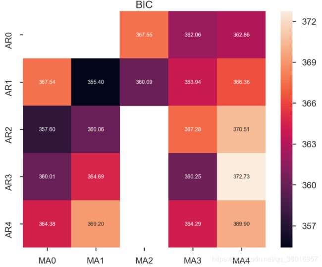
3、
由于p,q,d的不准确性,对p,q,d进行遍历,选择最好的参数
import itertools


p_min = 0
d_min = 0
q_min = 0
p_max = 4
d_max = 0
q_max = 4

#Initialize a DataFrame to store the results
results_bic = pd.DataFrame(index=['AR{}'.format(i) for i in range(p_min,p_max+1)],
                           columns=['MA{}'.format(i) for i in range(q_min,q_max+1)])

for p,d,q in itertools.product(range(p_min,p_max+1),
                               range(d_min,d_max+1),
                               range(q_min,q_max+1)):
    if p==0 and d==0 and q==0:
        results_bic.loc['AR{}'.format(p), 'MA{}'.format(q)] = np.nan
        continue

    try:
        model = sm.tsa.SARIMAX(ts_train, order=(p, d, q),
                               #enforce_stationarity=False,
                               #enforce_invertibility=False,
                              )
        results = model.fit()
        results_bic.loc['AR{}'.format(p), 'MA{}'.format(q)] = results.bic
    except:
        continue
results_bic = results_bic[results_bic.columns].astype(float)

fig, ax = plt.subplots(figsize=(10, 8))
ax = sns.heatmap(results_bic,
                 mask=results_bic.isnull(),
                 ax=ax,
                 annot=True,
                 fmt='.2f',
                 );
ax.set_title('BIC');

train_results = sm.tsa.arma_order_select_ic(ts_train, ic=['aic', 'bic'], trend='nc', max_ar=4, max_ma=4)
print('AIC', train_results.aic_min_order)
print('BIC', train_results.bic_min_order)
OUT:
AIC (4, 2)
BIC (1, 1)
4、数据切分
n_train=int(0.95*n_sample)+1
n_forecast=n_sample-n_train
#ts_df
ts_train = ts_df.iloc[:n_train]['value']
ts_test = ts_df.iloc[n_train:]['value']
5、arima模型建立
arima200 = sm.tsa.SARIMAX(ts_train, order=(2,0,0))#由order传入p,d,q
model_results = arima200.fit()
6、模型稳定性的判断
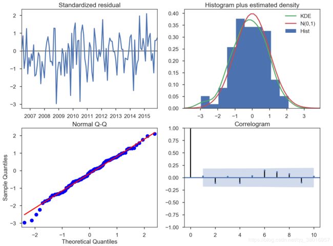
我们的主要关切是确保我们的模型的残差是不相关的,并且平均分布为零。 如果季节性ARIMA模型不能满足这些特性,这是一个很好的迹象,可以进一步改善。
残差在数理统计中是指实际观察值与估计值(拟合值)之间的差。“残差”蕴含了有关模型基本假设的重要信息。如果回归模型正确的话, 我们可以将残差看作误差的观测值。 它应符合模型的假设条件,且具有误差的一些性质。利用残差所提供的信息,来考察模型假设的合理性及数据的可靠性称为残差分析
在这种情况下,我们的模型诊断表明,模型残差正常分布如下:
-
在右上图中,我们看到红色KDE线与N(0,1)行(其中N(0,1) )是正态分布的标准符号,平均值0 ,标准偏差为1 ) 。 这是残留物正常分布的良好指示。
-
左下角的qq图显示,残差(蓝点)的有序分布遵循采用N(0, 1)的标准正态分布采样的线性趋势。 同样,这是残留物正常分布的强烈指示。
-
随着时间的推移(左上图)的残差不会显示任何明显的季节性,似乎是白噪声。 这通过右下角的自相关(即相关图)来证实,这表明时间序列残差与其本身的滞后版本具有低相关性。
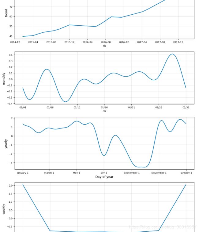
7、fbprophet框架
时间序列受四种成分影响:
-
趋势:宏观、长期、持续性的作用力,比如我国房地产价格;
-
周期:比如商品价格在较短时间内,围绕某个均值上下波动;
-
季节:变化规律相对固定,并呈现某种周期特征。比如每年国内航班的旅客数、空调销售量、每周晚高峰时间等。“季节”不一定按年计。每周、每天的不同时段的规律,也可称作季节性。
-
随机:随机的不确定性,比如10分钟内A股的股指变化,也是人们常说的随机过程(Stochastic Process)
Prophet所针对的,是Facebook的商业预测任务,这些任务一般具有以下特征:
按小时、日、周的观测值,至少是几个月的历史数据(最好是一年);
多种和人类活动相关的强周期性:比如每周的某日,一年中的某个时间;
按不确定间隔出现,已知的重要节假日,比如超级碗(Super Bowl);
合理数量的空白观测值或异常值;
时间趋势会转折,比如新产品发布;
非线性增长的趋势,比如到达了某种自然局限或饱和。
分析微软股票:
microsoft = Stocker('MSFT')  #MSFT股票名字,Stocker包含相关 函数
model, model_data = microsoft.create_prophet_model(days=0)  #预测未来days天
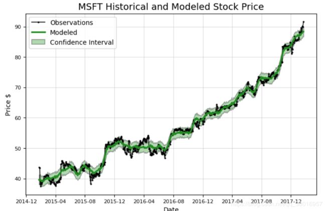
model.plot_components(model_data)
plt.show()
可分析时间段内的趋势:
分析亚马逊股票:
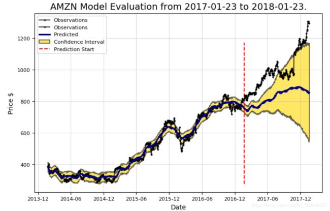
模型评估:
评估的指标包括:真实值和预测值之间的平均误差,上升与下降趋势,置信区间
amazon.evaluate_prediction()
OUT:
Prediction Range: 2017-01-23 to 2018-01-23.

Predicted price on 2018-01-20 = $855.17.
Actual price on    2018-01-19 = $1294.58.

Average Absolute Error on Training Data = $18.23.
Average Absolute Error on Testing  Data = $164.56.

When the model predicted an increase, the price increased 56.64% of the time.
When the model predicted a  decrease, the price decreased  43.81% of the time.

The actual value was within the 80% confidence interval 24.10% of the time.
优化:
Changepoint Prior Scale
该参数指定了突变点的权重,突变点就是那些突然上升,下降,或者是幅度突然变化明显的
权重大了,模型就会越符合于我们当前的训练数据集,但是过拟合也更大了。
权重小了,模型可能就欠拟合了,达不到我们预期的要求了。
选择了4组参数[0.001, 0.05, 0.1, 0.2]来观察结果
amazon.changepoint_prior_analysis(changepoint_priors=[0.001, 0.05, 0.1, 0.2])
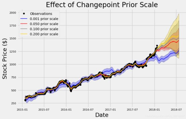
- 先来看蓝色的线,它的参数值设置的是最小的,看起来它在自己玩自己的,非常平均,但是欠拟合很明显
- 对于黄色的线,它非常接近于我们的训练数据集,层次鲜明,但是过拟合问题又很头疼
- 默认的参数是0.05,它在中间位置
评估
根据训练集预测的的误差,测试集预测的误差进行评估
amazon.changepoint_prior_validation(start_date='2016-01-04', end_date='2017-01-03', changepoint_priors=[0.001, 0.05, 0.1, 0.2])
OUT:
Validation Range 2016-01-04 to 2017-01-03.

     cps  train_err  train_range    test_err  test_range
0  0.001  44.475809   152.841613  149.373638  152.841541
1  0.050  11.203019    35.788779  152.033810  140.260382
2  0.100  10.722908    34.650575  152.903481  179.199686
3  0.200   9.725255    31.909034  127.604543  329.325001

咱们来试试更大的突变点值
amazon.changepoint_prior_validation(start_date='2016-01-04', end_date='2017-01-03', changepoint_priors=[0.25,0.4, 0.5, 0.6,0.7,0.8])

Validation Range 2016-01-04 to 2017-01-03.
OUT:
    cps  train_err  train_range    test_err   test_range
0  0.25   9.252699    30.686445  114.198811   451.654025
1  0.40   8.546549    28.809594   78.462455   768.760178
2  0.50   8.421606    28.542588   72.964334   819.560631
3  0.60   8.253096    28.000743   66.301627   949.097852
4  0.70   8.177868    27.857483   66.585793   920.312754
5  0.80   8.142373    27.763866   67.160883  1013.350436
