cs231n作业1--SVM
SVM算法:
1、算法思想:寻找一个超平面来划分不同类别的数据。http://www.cnblogs.com/end/p/3848740.html用图表很好的解释了什么是SVM
2、损失函数公式:
![]() 表示每个样本分类的损失值
表示每个样本分类的损失值
![]() 对所有测试样本的平均损失值
对所有测试样本的平均损失值
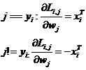
3、求导(梯度公式) :

在代码理解过程中遇到了一些问题,为什么一个样本对每个分类都要重复计算一遍第二个公式,这是因为在每一个样本进行损失值计算时,对其他所有非真实类都进行了损失值计算。比如有10个类,就需要计算9次损失函数公式中的第一个公式,相应的在计算梯度过程中就需要叠加计算9次梯度公式中的第一个公式。
4、代码实现:
linear_svm.py:
import numpy as np
from random import shuffle
from past.builtins import xrange

def svm_loss_naive(W, X, y, reg):
  """
  Structured SVM loss function, naive implementation (with loops).

  Inputs have dimension D, there are C classes, and we operate on minibatches
  of N examples.

  Inputs:
  - W: A numpy array of shape (D, C) containing weights.
  - X: A numpy array of shape (N, D) containing a minibatch of data.
  - y: A numpy array of shape (N,) containing training labels; y[i] = c means
    that X[i] has label c, where 0 <= c < C.
  - reg: (float) regularization strength

  Returns a tuple of:
  - loss as single float
  - gradient with respect to weights W; an array of same shape as W
  """
  dW = np.zeros(W.shape) # initialize the gradient as zero

  # compute the loss and the gradient
  num_classes = W.shape[1]
  num_train = X.shape[0]
  loss = 0.0
  for i in xrange(num_train):
    scores = X[i].dot(W)
    correct_class_score = scores[y[i]]
    for j in xrange(num_classes):
      if j == y[i]:
        continue
      margin = scores[j] - correct_class_score + 1 # note delta = 1
      if margin > 0:
        loss += margin
        dW[:,y[i]] += -X[i,:]
        dW[:,j] += X[i,:]

  # Right now the loss is a sum over all training examples, but we want it
  # to be an average instead so we divide by num_train.
  loss /= num_train
  dW /=num_train     #

  # Add regularization to the loss.
  loss += 0.5 * reg * np.sum(W * W)

  dW += reg * W

  #############################################################################
  # TODO:                                                                     #
  # Compute the gradient of the loss function and store it dW.                #
  # Rather that first computing the loss and then computing the derivative,   #
  # it may be simpler to compute the derivative at the same time that the     #
  # loss is being computed. As a result you may need to modify some of the    #
  # code above to compute the gradient.                                       #
  #############################################################################

  return loss, dW


def svm_loss_vectorized(W, X, y, reg):
  """
  Structured SVM loss function, vectorized implementation.

  Inputs and outputs are the same as svm_loss_naive.
  """
  loss = 0.0
  dW = np.zeros(W.shape) # initialize the gradient as zero

  #############################################################################
  # TODO:                                                                     #
  # Implement a vectorized version of the structured SVM loss, storing the    #
  # result in loss.                                                           #
  #############################################################################
  scores = X.dot(W)
  num_train = X.shape[0]
  num_classes = W.shape[1]
  scores_correct = scores[np.arange(num_train), y]
  scores_correct = np.reshape(scores_correct, (num_train, 1))
  margins = scores - scores_correct + 1.0
  margins[np.arange(num_train), y] = 0.0
  margins[margins <= 0] = 0.0
  loss += np.sum(margins) / num_train
  loss += 0.5 * reg * np.sum(W * W)

  #############################################################################
  #                             END OF YOUR CODE                              #
  #############################################################################

  #############################################################################
  # TODO:                                                                     #
  # Implement a vectorized version of the gradient for the structured SVM     #
  # loss, storing the result in dW.                                           #
  #                                                                           #
  # Hint: Instead of computing the gradient from scratch, it may be easier    #
  # to reuse some of the intermediate values that you used to compute the     #
  # loss.                                                                     #
  #############################################################################
  # compute the gradient
  margins[margins > 0] = 1.0
  row_sum = np.sum(margins, axis=1)
  margins[np.arange(num_train), y] = -row_sum
  dW += np.dot(X.T, margins)/num_train + reg * W
  #############################################################################
  #                             END OF YOUR CODE                              #
  #############################################################################

  return loss, dW
svm.ipynb
# Use the validation set to tune hyperparameters (regularization strength and
# learning rate). You should experiment with different ranges for the learning
# rates and regularization strengths; if you are careful you should be able to
# get a classification accuracy of about 0.4 on the validation set.
learning_rates = [1e-7, 5e-5]
regularization_strengths = [2.5e4, 5e4]

# results is dictionary mapping tuples of the form
# (learning_rate, regularization_strength) to tuples of the form
# (training_accuracy, validation_accuracy). The accuracy is simply the fraction
# of data points that are correctly classified.
results = {}
best_val = -1   # The highest validation accuracy that we have seen so far.
best_svm = None # The LinearSVM object that achieved the highest validation rate.

################################################################################
# TODO:                                                                        #
# Write code that chooses the best hyperparameters by tuning on the validation #
# set. For each combination of hyperparameters, train a linear SVM on the      #
# training set, compute its accuracy on the training and validation sets, and  #
# store these numbers in the results dictionary. In addition, store the best   #
# validation accuracy in best_val and the LinearSVM object that achieves this  #
# accuracy in best_svm.                                                        #
#                                                                              #
# Hint: You should use a small value for num_iters as you develop your         #
# validation code so that the SVMs don't take much time to train; once you are #
# confident that your validation code works, you should rerun the validation   #
# code with a larger value for num_iters.                                      #
################################################################################
iters = 2000 #100
for lr in learning_rates:
    for rs in regularization_strengths:
        svm = LinearSVM()
        svm.train(X_train, y_train, learning_rate=lr, reg=rs, num_iters=iters)

        y_train_pred = svm.predict(X_train)
        acc_train = np.mean(y_train == y_train_pred)
        y_val_pred = svm.predict(X_val)
        acc_val = np.mean(y_val == y_val_pred)

        results[(lr, rs)] = (acc_train, acc_val)

        if best_val < acc_val:
            best_val = acc_val
            best_svm = svm
################################################################################
#                              END OF YOUR CODE                                #
################################################################################

# Print out results.
for lr, reg in sorted(results):
    train_accuracy, val_accuracy = results[(lr, reg)]
    print('lr %e reg %e train accuracy: %f val accuracy: %f' % (
                lr, reg, train_accuracy, val_accuracy))

print('best validation accuracy achieved during cross-validation: %f' % best_val)