基于低秩矩阵的的图像显著性检测
如果矩阵的秩远远小于其行数或者列数,那么这类矩阵就称为低秩矩阵。低秩分解的基本思想是:若输入数据矩阵是由两种特征比较明显的数据或组成部分,其中一种成分的数据矩阵具有稀疏特性而另一种具有低秩特性,那么该矩阵就可以通过凸优化方法恢复出低秩成分和稀疏成分。因此,通过低秩分解可以将图像背景近似地表示为一个低秩矩阵,使用稀疏部分代表完成背景冗余信息和前景显著目标的分离。
全局低秩显著性检测算法
全局低秩显著性检测算法首先根据自然图像前景目标和背景亮度、颜色的差异性重构出图像前景显著目标;然后利用低秩分解对图像中的非显著性区域进行抑制。
提取对比度
计算CIE*Lab颜色空间三通道图像与其均值之差的绝对值。由下式的到:
式中j的取值为1,2,3表示CIE*Lab颜色空间的三个颜色通道;I
cj
表示j通道均值之差的绝对值,表示j通道对比度特征。
获取初始显著图
根据上式计算所得三通道对比度特征分别取出标准差最大的I'cj和二维熵最小的I'‘cj,通过权重融合的到初始显著图具体计算方法如下:
![]()
其中Ic为所得初始显著图。标准差主要衡量数据值偏离算数平均值的程度。标准差越大,这些值的偏离平均值就越大。在本文的图像显著性检测算法中,若标准差越大则认为其与背景的差异性越大,显著性越高。具体计算如下:

式中S为图像矩阵的标准差,N为像素点的个数,Xi为第i个像素点的值,![]() 为图像矩阵的均值。
为图像矩阵的均值。
图像的二维信息熵相比图像的一维信息熵考虑了图像中的空间信息。计算如下:
![]()
gn表示为高斯滤波器,x为二维图像信号,其原理是首先对输入二维信号经过高斯滤波消除空间位置信息的干扰后再计算其信息熵,显著图的熵越小说明其显著程度越高。
使用标准差最大和二维熵最小的两个指标加权得到的初始显著图如下:
全局低秩分解
对得到的初始显著图进行低秩分解,得到初始显著图的低秩部分和稀疏部分,计算方法如下:
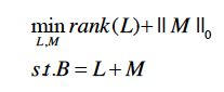
式中:B为输入图像矩阵,L和M分别对应于抵制和稀疏部分。||M||
0表示M的L0范数。(L0范数是指向量中非0的元素的个数。如果我们用L0范数来规则化一个参数矩阵M的话,就是希望M的大部分元素都是0。)由于这是一个NP-Hard问题,所以可以转化为求解如下优化问题:
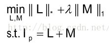
式中I
p
为初始显著图,L为低秩矩阵对应于图像背景冗余部分,M为稀疏矩阵对应于图像前景显著目标, 为系数平衡低秩和稀疏两部分。当它取值过大时,一些前景目标信息会被当做背景处理;反之当系数取值较小时,一些背景信息会被当做前景目标处理。用初始显著图减去分解之后的低秩部分得到全局显著图。

式中I
g
表示全局显著图,Ip为初始显著图。
matlab实现
(1)RGB色彩空间和Lab色彩空间的转换
function [R, G, B] = Lab2RGB(L, a, b)
%LAB2RGB Convert an image from CIELAB to RGB
%
% function [R, G, B] = Lab2RGB(L, a, b)
% function [R, G, B] = Lab2RGB(I)
% function I = Lab2RGB(...)
%
% Lab2RGB takes L, a, and b double matrices, or an M x N x 3 double
% image, and returns an image in the RGB color space.  Values for L are in
% the range [0,100] while a* and b* are roughly in the range [-110,110].
% If 3 outputs are specified, the values will be returned as doubles in the
% range [0,1], otherwise the values will be uint8s in the range [0,255].
%
% This transform is based on ITU-R Recommendation BT.709 using the D65
% white point reference. The error in transforming RGB -> Lab -> RGB is
% approximately 10^-5.
%
% See also RGB2LAB.

% By Mark Ruzon from C code by Yossi Rubner, 23 September 1997.
% Updated for MATLAB 5 28 January 1998.
% Fixed a bug in conversion back to uint8 9 September 1999.
% Updated for MATLAB 7 30 March 2009.

if nargin == 1
  b = L(:,:,3);
  a = L(:,:,2);
  L = L(:,:,1);
end

% Thresholds
T1 = 0.008856;
T2 = 0.206893;

[M, N] = size(L);
s = M * N;
L = reshape(L, 1, s);
a = reshape(a, 1, s);
b = reshape(b, 1, s);

% Compute Y
fY = ((L + 16) / 116) .^ 3;
YT = fY > T1;
fY = (~YT) .* (L / 903.3) + YT .* fY;
Y = fY;

% Alter fY slightly for further calculations
fY = YT .* (fY .^ (1/3)) + (~YT) .* (7.787 .* fY + 16/116);

% Compute X
fX = a / 500 + fY;
XT = fX > T2;
X = (XT .* (fX .^ 3) + (~XT) .* ((fX - 16/116) / 7.787));

% Compute Z
fZ = fY - b / 200;
ZT = fZ > T2;
Z = (ZT .* (fZ .^ 3) + (~ZT) .* ((fZ - 16/116) / 7.787));

% Normalize for D65 white point
X = X * 0.950456;
Z = Z * 1.088754;

% XYZ to RGB
MAT = [ 3.240479 -1.537150 -0.498535;
       -0.969256  1.875992  0.041556;
        0.055648 -0.204043  1.057311];

RGB = max(min(MAT * [X; Y; Z], 1), 0);

R = reshape(RGB(1,:), M, N);
G = reshape(RGB(2,:), M, N);
B = reshape(RGB(3,:), M, N);

if nargout < 2
  R = uint8(round(cat(3,R,G,B) * 255));
end
function [L,a,b] = RGB2Lab(R,G,B)
%RGB2LAB Convert an image from RGB to CIELAB
%
% function [L, a, b] = RGB2Lab(R, G, B)
% function [L, a, b] = RGB2Lab(I)
% function I = RGB2Lab(...)
%
% RGB2Lab takes red, green, and blue matrices, or a single M x N x 3 image,
% and returns an image in the CIELAB color space.  RGB values can be
% either between 0 and 1 or between 0 and 255.  Values for L are in the
% range [0,100] while a and b are roughly in the range [-110,110].  The
% output is of type double.
%
% This transform is based on ITU-R Recommendation BT.709 using the D65
% white point reference. The error in transforming RGB -> Lab -> RGB is
% approximately 10^-5.
%
% See also LAB2RGB.

% By Mark Ruzon from C code by Yossi Rubner, 23 September 1997.
% Updated for MATLAB 5 28 January 1998.
% Updated for MATLAB 7 30 March 2009.

if nargin == 1
  B = double(R(:,:,3));
  G = double(R(:,:,2));
  R = double(R(:,:,1));
end

if max(max(R)) > 1.0 || max(max(G)) > 1.0 || max(max(B)) > 1.0
  R = double(R) / 255;
  G = double(G) / 255;
  B = double(B) / 255;
end

% Set a threshold
T = 0.008856;

[M, N] = size(R);
s = M * N;
RGB = [reshape(R,1,s); reshape(G,1,s); reshape(B,1,s)];

% RGB to XYZ
MAT = [0.412453 0.357580 0.180423;
       0.212671 0.715160 0.072169;
       0.019334 0.119193 0.950227];
XYZ = MAT * RGB;

% Normalize for D65 white point
X = XYZ(1,:) / 0.950456;
Y = XYZ(2,:);
Z = XYZ(3,:) / 1.088754;

XT = X > T;
YT = Y > T;
ZT = Z > T;

Y3 = Y.^(1/3);

fX = XT .* X.^(1/3) + (~XT) .* (7.787 .* X + 16/116);
fY = YT .* Y3 + (~YT) .* (7.787 .* Y + 16/116);
fZ = ZT .* Z.^(1/3) + (~ZT) .* (7.787 .* Z + 16/116);

L = reshape(YT .* (116 * Y3 - 16.0) + (~YT) .* (903.3 * Y), M, N);
a = reshape(500 * (fX - fY), M, N);
b = reshape(200 * (fY - fZ), M, N);

if nargout < 2
  L = cat(3,L,a,b);
end
(2)获取初始显著图
%导入需要处理的图片
I=imread('4_140_140766.jpg');
I=imresize(I,[300 300]);
I1=RGB2Lab(I);
L1 = double(I1(:,:,1));  L2 = double(I1(:,:,2)); L3 = double(I1(:,:,3));
PL1=mean(L1(:));
PL2=mean(L2(:));
PL3=mean(L3(:));
[m,n]=size(L1);
for i=1:m
for j=1:n
LL1(i,j)=abs(L1(i,j)-PL1);
end
end


for i=1:m
for j=1:n
LL2(i,j)=abs(L2(i,j)-PL2);
end
end


for i=1:m
for j=1:n
LL3(i,j)=abs(L3(i,j)-PL3);
end
end

LLL1=reshape(LL1,1,[]);
SL1=std(LLL1);
LLL2=reshape(LL2,1,[]);
SL2=std(LLL2);
LLL3=reshape(LL3,1,[]);
SL3=std(LLL3);

%比较标准差最大
SL=max(max(SL1,SL2),SL3);

 G = fspecial('gaussian', [5 5], 1);
 GL1=imfilter(LL1, G, 'circular');
 hist=imhist(GL1)/prod(size(GL1));
G1=find(hist);
H1=-hist(G1)'*log2(hist(G1));

GL2=imfilter(LL2, G, 'circular');
hist=imhist(GL2)/prod(size(GL2));
G2=find(hist);
H2=-hist(G2)'*log2(hist(G2));

GL3=imfilter(LL3, G, 'circular');
hist=imhist(GL3)/prod(size(GL3));
G3=find(hist);
H3=-hist(G3)'*log2(hist(G3));

%比较二维熵最小的
H=min(min(H1,H2),H3);

if(SL==SL1)
    ZL=LL1;
end
if(SL==SL2)
    ZL=LL2;
end
if(SL==SL3)
    ZL=LL3;
end

if(H==H1)
    HL=LL1;
end
if(H==H2)
    HL=LL2;
end
if(H==H3)
    HL=LL3;
end

%计算初始显著图
 C=0.35*ZL+0.65*HL;
(3)低秩分解部分代码
function [Z,E] = lrr(X,lambda)
% This routine solves the following nuclear-norm optimization problem
% by using inexact Augmented Lagrange Multiplier(增广拉格朗日乘子法), which has been also presented
% in the paper entitled "Robust Subspace Segmentation
% by Low-Rank Representation".
%------------------------------
% min |Z|_*+lambda*|E|_2,1
% s.t., X = XZ+E
%--------------------------------
% inputs:
%        X -- D*N data matrix, D is the data dimension, and N is the number
%             of data vectors.
if nargin<2
    lambda = 1;
end
tol = 1e-8;
maxIter = 1e6;
% X=rgb2gray(X);
% X=double(X);
[d n] = size(X);
% n=min(d,n);
% X=imresize(X,[n n]);
rho = 1.1;
max_mu = 1e30;
mu = 1e-2;
xtx = X'*X;
inv_x = inv(xtx+eye(n));
%% Initializing optimization variables
% intialize
J = zeros(n,n);
Z = zeros(n,n);
E = sparse(d,n);

Y1 = zeros(d,n);
Y2 = zeros(n,n);
%% Start main loop
iter = 0;
disp(['initial,rank=' num2str(rank(Z))]);
while iter1/mu));
    if svp>=1
        sigma = sigma(1:svp)-1/mu;
    else
        svp = 1;
        sigma = 0;
    end
    J = U(:,1:svp)*diag(sigma)*V(:,1:svp)';

    Z = inv_x*(xtx-X'*E+J+(X'*Y1-Y2)/mu);

    xmaz = X-X*Z;
    temp = X-X*Z+Y1/mu;
    E = solve_l1l2(temp,lambda/mu);

    leq1 = xmaz-E;
    leq2 = Z-J;
    stopC = max(max(max(abs(leq1))),max(max(abs(leq2))));
    if iter==1 || mod(iter,50)==0 || stopClambda
    x = (nw-lambda)*w/nw;
else
    x = zeros(length(w),1);
end
(4)主函数调用部分
  [Z E]=lrr(C,0.01);%全局低秩Z为低秩部分E为稀疏部分
  ZZ=(C-Z).*C;
  figure,imshow(ZZ,[]);
实验结果
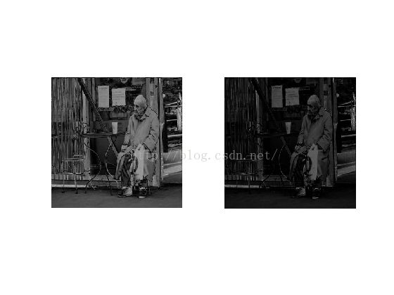
原图像和全局低秩分解结果对比
利用四元相位谱残差显著性检测的结果与结合全局低秩分解和四元相位谱残差的显著性检测结果对比
