SoSH Project
SoSH Project
http://solar-center.stanford.edu/SoSH/
SoSH Project
Sonification of Solar Harmonics
About
The Sun is a resonant cavity for very low frequency acoustic waves, and just like a musical instrument, it supports a number of oscillation modes, also commonly known as harmonics. We are able to observe these harmonics by looking at how the Sun's surface oscillates in response to them. Although this data has been studied scientifically for decades, it has only rarely been sonified, which is the process of rendering data as audible sound.
The Sonification of Solar Harmonics (SoSH) Project seeks to sonify data related to the field of helioseismology and distribute tools for others to do the same. The software package is built on Pure Data, a freely available graphical interface for audio processing. Extensive documentation of the project can be found in this PDF. A supplemental software package, written in Python, is available to create visualizations of solar harmonics. Its documentation can be found here.
Helioseismology
The study of acoustic waves inside the Sun is called helioseismology; an overview can be found here. In short, turbulent convection (boiling) near the surface excites sound waves. The waves with frequencies that resonate form the harmonics. Then, just as the frequency of a plucked guitar string gets higher with more tension and lower with greater thickness, the frequencies of the Sun's harmonics enable us to infer properties of the solar interior such as its pressure and density.
What does a harmonic (a mode) on the Sun look like? To begin with, it is a mathematical theorem that any arbitrary shape of the Sun's surface can be expressed as a sum over its harmonics (this is also true for a guitar string). In the case of the Sun, we call them spherical harmonics, and each of them are labelled by two integers: the spherical harmonic degree l (ell) and the azimuthal order m. The degree l is equal to or greater than zero, and for each l, there are 2*l+1 values of m, ranging from -l to l.
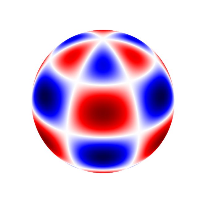
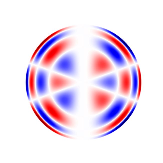
One way to understand spherical harmonics is in terms of their node lines, which are the places on the sphere where the spherical harmonics are zero. The degree l tells how many of these node lines there are in total, and the absolute value of the order |m| gives the number in longitude, so the number of node lines in latitude is l - |m|. Therefore a spherical harmonic with m = 0 has only latitudinal bands, while one with m = l has only sections like an orange. A third integer, the radial order n, tells how many nodes the oscillation has along the Sun's radius. Since only the surface of the Sun is visible to us, all the values of n are present in each spherical harmonic labelled by l and m, although only some of them will be excited to any appreciable amplitude. The total mode, then, is represented as a product of a spherical harmonic, which is a function of latitude and longitude, and another function of radius.
The figures below illustrate two examples of modes with degree 5 and all the allowable values of m. Modes with m < 0 are not included because they are indistinguishable from modes with m > 0 at this stage; negative values of m are discussed in the Visualizations section below. For clarity, we have shown n = 3, although in practice this mode lies below the minimum frequency we are able to measure. Closer to the peak in acoustic power at 3000 microhertz is the next mode shown, n = 20. At this frequency, the nodes along the radius become so closely spaced near the surface that they are difficult to discern at this scale. It is important to realize that we are seeing modes of many different n in each spherical harmonic. For instance, for degree 5 we might measure modes with n ranging from 7 to 28, each oscillating at its own frequency, roughly 140 microhertz apart from each other.
Surface View
l = 5, m = 0
l = 5, m = 1
l = 5, m = 2
l = 5, m = 3
l = 5, m = 4
l = 5, m = 5
Interior View, n=3, frequency = 800 microhertz
l = 5, m = 0
l = 5, m = 1
l = 5, m = 2
l = 5, m = 3
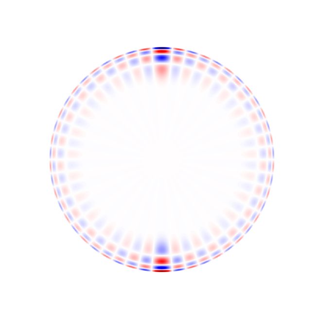
l = 5, m = 4
l = 5, m = 5
Interior View, n=20, frequency = 3190 microhertz
l = 5, m = 0
l = 5, m = 1
l = 5, m = 2
l = 5, m = 3
l = 5, m = 4
l = 5, m = 5
Each mode oscillates with its characteristic frequency, and each samples different regions of the Sun. At a given degree, high frequencies will penetrate more deeply, while low frequencies are trapped closer to the surface. Likewise, at a given frequency, high values of the degree l will be trapped near the surface, while low values will penetrate almost all the way to the core, with l = 0 even reaching the center. This is further illustrated in the next series of figures below, which show a selection of modes with degree l = 25 for the same two values of n.
Different modes also sample different latitudes, according to the value of |m| relative to the degree l. Modes with high absolute values of m have their maximum amplitude at low latitudes, whereas lower values extend to higher latitudes. It is because the different modes sample different regions of the Sun that we are able to use their frequencies to determine solar properties as a function of both depth and latitude.
Surface View
l = 25, m = 0
l = 25, m = 5
l = 25, m = 10
l = 25, m = 15
l = 25, m = 20
l = 25, m = 25
Interior View, n=3, frequency = 1290 microhertz
l = 25, m = 0
l = 25, m = 5
l = 25, m = 10
l = 25, m = 15
l = 25, m = 20
l = 25, m = 25
Interior View, n=20, frequency = 3990 microhertz
l = 25, m = 0
l = 25, m = 5
l = 25, m = 10
l = 25, m = 15
l = 25, m = 20
l = 25, m = 25
To determine the frequencies of the Sun's harmonics, the instruments we discuss here take data for 72 days. For each image produced, we decompose it into its various spherical harmonic components. For each of these components, we form a timeseries of its amplitude. From the timeseries we are able to construct the power spectrum (acoustic power as a function of frequency). The location of peaks in the power spectrum correspond to the frequencies of the modes (harmonics). The height of the peak tells us the mode amplitude, and the width of the peak tells us how much the oscillation is damped. Each n will have its own peak in the power spectrum.
The relationship between l, n, and frequency is illustrated in the next figure below. Plotted on the left is raw power as a function of l and frequency for m = 0. As one can see, the modes for a given n form a ridge of power. The right panel is a scatter plot indicating which modes we have been able to successfully fit. In both plots the bottom ridge corresponds to n = 0.
SoSH Tool
The strongest of the Sun's harmonics have periods of about 5 minutes, corresponding to frequencies of only about 0.003 hertz. Unfortunately, this is far below the range of human hearing, which is typically taken to be 20 - 20,000 hertz, although most people are only sensitive to a smaller range. Hence, if we would like to experience the sound of the Sun with our ears, these very low sounds must be scaled to the range we can hear.
The most straightforward way to do so would be to use the spherical harmonic timeseries we already have in hand and speed them up. But by how much? The answer of course is arbitrary and will depend on your preference, but as long as this choice is applied consistently you will still be able to hear the real relationship between different solar tones.
Let us suppose that we want to transpose a mode in the peak power range at about 0.003 hertz up to 300 hertz; this amounts to speeding up the timeseries by a factor of 100,000. If an instrument produces an image once a minute, then 72 days of data amounts to 103,680 data points, or samples. It is easy to see that in this case the sped-up timeseries would now play in just over a minute. One must also consider the sample rate, however, or the rate at which audio is played back. Speeding up the original sample rate of (1/60) hertz by a factor of 100,000 yields a new sample rate of 1666.67 hertz, and one unfortunately finds very few audio players that will play any sample rate less than 8000 hertz. Assuming this sample rate, our 0.003 hertz mode on the Sun will now be transposed up to 1440 hertz and the timeseries will play in about 13 seconds.
But suppose you want to play it in a shorter time; 13 seconds is a long time to sound a single note, although you might want to do so in some circumstances. You could increase the sample rate further still, but at some point the mode will be transposed to an uncomfortably high frequency. To understand the solution to this problem, we must explore the process by which we shall isolate the modes.
At this point in our processing, playing an unfiltered timeseries would sound just like static, or noise. This is because very many modes are sounding simultaneously in any given timeseries, not to mention the background noise involved in our observation of the modes. Therefore, if we want to isolate a single mode, we have to do some filtering. Luckily, as mentioned above, we have already measured the frequency, amplitude, and width of many modes. We can use these parameters, or mode fits as they are called, to pick out the particular part of the power spectrum corresponding to a single mode, and set the rest of the power spectrum artificially to zero. We then transform back into a function of time so that we can play the filtered data back as a timeseries.
Since we are selecting only a narrow range of frequencies, we have the freedom to shift the entire power spectrum down in frequency before we transform back to timeseries. This timeseries will play in the same amount of time as before, but the frequencies in it will be transposed down by the same factor that we shifted the power spectrum. For every power of 2 shifted down, the tone will drop by one octave.
One approach might be to decide how long you want to sound each tone (keeping in mind that looping is also an option). This will determine the sample rate at which you will play the timeseries. Then you can choose a downshift factor to suit yourself. As long as you use the same sample rate and downshift factor when you sonify every mode, the frequency relationships between them will be preserved. In other words, you will hear the same musical intervals as you would on the Sun.
Screenshots
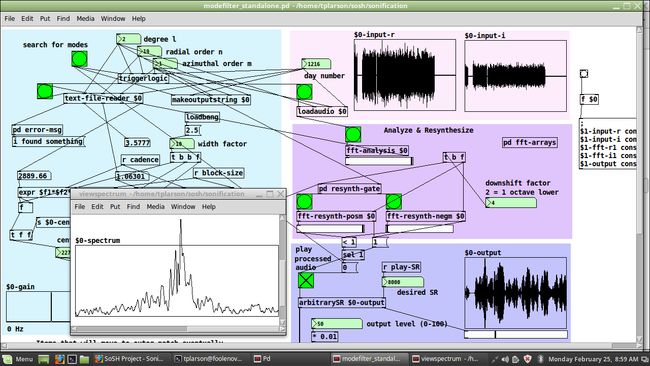
Below are some screenshots of the SoSH Tool. A program in Pure Data is called a "patch". The first example shown is the basic patch, modefilter_standalone.pd:
One can see where we have entered the day number and the mode's l, n, and m at the top of the patch. The input is shown at top right, and the output is displayed at bottom right. The "viewspectrum" window shows the small piece of the power spectrum we used to generate that output.
Next we show how this patch is converted to a subpatch called "modefilter" to be used in the parent patch example_sum.pd:
We have used 5 instances of the new subpatch so that we may sound 5 tones at once or in sequence using the interface on the right edge of the patch. The pink toggles have been enlarged for ease of use with a touchscreen. One may still click on the individual instances of modefilter to interact with them directly, for instance to view their input and output. The different modes may be summed into a single array "sumhold" which may then be written to disk.
Finally, we show the most general patch included with the SoSH Tool, example_sequencer.pd. It is able to create sums of modes like the patch above, but using only a single instance of modefilter. It applies a windowing function to the finished sum and then concatenates the result onto a longer array, which can then be played back:
The entire sequence is controlled by a simple text file read by the "qlist" object. However, this patch may also be used entirely interactively, just like the first patch shown above.
Sound Samples
Here are some examples we have created using the SoSH Tool. For a description of the Michelson Doppler Imager (MDI) and the Helioseismic and Magnetic Imager (HMI), see the section on data below; the important point is that MDI has a native sample rate 3/4 that of HMI.
- Three Modes (1.6 MB)
Three modes are represented in this file: n=3-5 for l=150 and m=0. They first sound in sequence and then simultaneously. The data was taken by MDI starting at day number 6328. At a sample rate of 12 kHz and a downshift factor of 8, the total transposition factor is 90,000. The file then plays in about 35.6 seconds and the tones become 224.4, 253.1 and 280.5 Hz. The difference in volume for each mode corresponds to its amplitude as measured on the Sun.
- Solar Rotation (1.6 MB)
This file contains two modes with l=20 and n=16, one at m=-20 and one at m=20. Again, they sound first in sequence and then simultaneously. The data was taken by HMI starting at day number 6328. At a same sample rate of 16 kHz and a downshift factor of 8, the total transposition factor becomes 120,000. The file plays in 26 seconds and the modes are transposed up to 368.6 and 370.8 Hz. These tones are likely too close to distinguish, but solar rotation is audible as the 2.2 Hz beat frequency when they play together.
- MDI: Two Modes (31 MB)
This file spans the entire MDI mission and is the sum of two modes: n=17 and 21 for l=5, m=3. At a sample rate of 9 kHz, this file plays in about 14.6 minutes. A downshift factor of 4 was applied. The intervals of silence in this file represent times when MDI was not operational.
- HMI: Two Modes (24 MB)
This file spans the first 8.5 years of the HMI mission and sums the same two modes as above. At a same sample rate of 12 kHz, this file plays in about 8.45 minutes. The same downshift factor of 4 was applied.
- Effect of Filter Width (2.4 MB)
The frequency filter used to create this file is centered on the mode with l=5, m=3 and n=19. The data was taken by MDI starting at day number 6328. It is filtered first with a width of 5 times the mode linewidth, then 10, 20, 40 and 80 this amount, separated in the file by intervals of silence. A sample rate of 10 kHz and downshift of 5 was used. At 40 times the linewidth you can hear one adjacent mode, and at 80 you can hear several.
Visualizations
Several of the above graphics were created using the SoshPy Visualization Package. Here we must emphasize an important distinction between the SoSH tool and the visualizations. While the the audio part of the project reads real solar data and uses actual measurements to render it as audible sound, the visualizations are based on models only. The model data cannot tell us how the mode parameters vary with time, nor how the Sun rotates, but on the other hand we can model many more modes than we are able to measure. Both approaches are important in helioseismology. We call the creation of a model a forward problem: starting from some assumptions about the physics inside the Sun, we predict mode characteristics such as their frequency and amplitude. The opposite is called an inverse problem: starting from measurements, primarily of mode frequencies, we try to infer the properties of the solar interior.
Of course a model is still needed to make these inferences, but rather than assuming the parameters of this model, we constrain them using the observations. Put another way, we make guesses about what is going on inside the Sun, and this allows us to guess what the mode frequencies would be. Then we use surface observations to measure the actual frequencies, and this allows us to modify the guesses we made about the interior. The visualizations we present here are an example of solutions to a forward problem, and listening to the audio renderings is the first part of an inverse problem.
Helioseismology, Extended Discussion
So far, we have subtly omitted the manner in which we make these observations, as well as the specific quantity we have shown in the visualizations. Recall that we are here concerned with sound, which is simply the coherent vibration of matter. Now imagine a plasma element (a chunk of matter) at the surface of the Sun. In response to a given mode, which inhabits the entire Sun, this single plasma element will oscillate at the mode frequency. In other words, it moves back and forth; some part of this motion will be in the radial direction, some in the latitudinal direction, and some in the longitudinal direction. A model can tell us how much of the motion lies in each direction. We call the radial motion the vertical displacement, and we put the latitudinal and longitudinal components of the motion together to make the horizontal displacement.
Now, how are we to measure this displacement? Actually, it turns out to be much easier to measure the speed of our plasma element, which is simply the rate at which the displacment is changing. In mathematical terms, we say the velocity of the plasma element is the derivative of its position. Since the plasma element is moving in response to one of the Sun's harmonics, it can be modeled as a simple harmonic oscillator. In other words, its motion is mathematically equivalent to the motion of a weight attached to a spring. In particular, the model tells us that the magnitude of the the plasma element's velocity is equal to the magnitude of its displacement multiplied by its frequency, which is simply the mode frequency.
It is the velocity of the plasma element that we are able to measure. The details of this measurement are beyond the scope of this discussion, but in short we are actually measuring the frequency of spectral lines of atoms at the solar surface. For plasma at rest, these spectral lines have precise frequencies that can be measured in a laboratory. The motion of the plasma causes these frequencies to be shifted slightly. This is called the Doppler Effect, and it is exactly the same phenomenon that you can observe with sound waves when a siren drives past: when the siren is approaching it sounds higher, and when it is moving away it sounds lower. We use the Doppler Effect to create velocity images of the Sun's surface, and for this reason we call them dopplergrams. Each pixel of the image corresponds to one of our plasma elements, and the pixel value tells us how fast that element is moving toward or away from the observer.
Here we run into a fundamental limitation of our method of observation. We would like to know both the vertical and horizontal components of the velocity. Unfortunately, a dopplergram only gives us the velocity along the observer's line of sight. At the center of the solar image, this is exactly the vertical component, and at the very edge, it is the horizontal component. Everywhere else we measure a mix of the two, and nowhere can we measure both of them. This is one of the reasons we have to rely on a model.
So what exactly have we plotted in the figures above? It turns out that for a large majority of modes, the horizontal component is very small compared to the vertical component at the surface, and for many purposes can be neglected entirely. Hence, in the plots above we have shown the vertical component of the velocity only. Properly speaking, this is the only quantity given directly by a spherical harmonic (more on this below). The SoshPy Visualization Package, however, is also able to plot the latitudinal and longitudinal components, as well as these two combined into the total horizontal component. It can also plot the magnitude of the total velocity, as well this magnitude squared.
Why squared, you ask? To answer this, we must consider the interior plots. In this case, we actually plot the velocities scaled by the square root of the density. This is for two reasons. Firstly, since the velocities drop off rapidly with depth while the density increases rapidly, the quantity plotted shows visible variations throughout the interior. Secondly, the square of this scaled velocity is actually equal to the energy density of the mode. Note that because the density of the background model is constant at the solar surface, the surface plots of the velocity squared look exactly like a plot of the energy density there.
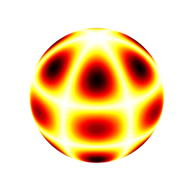
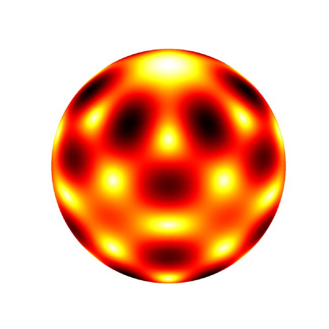
When plotting these variables, it is important to recognize that the three velocity components are signed quantities, which is to say that they range from positive to negative. The magnitudes and energy density, on the other hand, are strictly positive. Hence, we would usually use different colormaps for the two cases. For example, below we show surface and interior views of the radial, theta and phi components of the velocity using the same colormap as above.
l=5, m=3, n=3
Vr
Vt
Vp
Vr
Vt
Vp
As stated above, the radial component is given exactly by a spherical harmonic. The theta component is given by its derivative in latitude, and the phi component is given by a spherical harmonic scaled by cos(latitude) and shifted in longitude. In each case, the colormap is scaled to use the full range of the data. Next, we use a different colormap to show surface and interior views of the magnitude of the total velocity, its square, and the magnitude of the horizontal component. In both colormaps, the color white corresponds to a value of zero. You can see that because the radial component is so much larger than the horizontal components, the total velocity closely resembles the absolute value of the radial velocity.
l=5, m=3, n=3
Vmag
Vsq
Vh
Vmag
Vsq
Vh
By default the visualizations are also animated. It is here that we are able to distinguish between negative and positive values of the azimuthal order m. One sign of m will rotate in one direction, while the opposite sign rotates in the other. To see a non-rotating mode, we can plot the sum of a mode with one value of m and a second with its negative. It is because both signs of m look exactly alike that we are unable to separate them during the spherical harmonic decomposition of images; this can only be done in frequency space. The sign of m that rotates in the same direction that the Sun rotates will be shifted up in frequency, and the sign that goes against solar rotation will be shifted down in frequency. Furthermore, since the different modes sample different depths and latitudes as described above, we can use this frequency splitting in m, as it is called, to infer how solar rotation varies inside the Sun.
Surface Radial Velocity, l=5, |m|=3
m=+3
+
m=-3
=
|m|=3
As this example demonstrates, the SoshPy Visualization Package is also able to plot sums of modes. For single modes, the visualizations are animated at an arbitrary frequency such that the animation will loop seemlessly. For sums of modes, however, the actual model frequencies are used, scaled up by an arbitrary factor. Because in the model the frequency does not depend on m, we can still achieve a seemless loop when summing modes with the same l and n. For more general sums the loop will not be seemless, but one can select the scale factor as well as the number of frames in the animation to come close. Below we show some examples. Your browser may have difficulty playing many simultaneous animations; it might be necessary play them one at a time or even stop those playing above.
Surface Radial Velocity
l=6, m=±5, n=5
l=8, m=±4, n=5
l=9, m=±3, n=5
mp4
webm
l=6, m=±5, n=10
l=8, m=±4, n=15
l=9, m=±3, n=20
mp4
webm
l=12, m=±10, n=5
l=16, m=±8, n=5
l=18, m=±6, n=5
mp4
webm
l=12, m=±10, n=10
l=16, m=±8, n=15
l=18, m=±6, n=20
mp4
webm
Interior Radial Velocity
l=6, m=±5, n=5
l=8, m=±4, n=5
l=9, m=±3, n=5
mp4
webm
l=6, m=±5, n=10
l=8, m=±4, n=15
l=9, m=±3, n=20
mp4
webm
l=12, m=±10, n=5
l=16, m=±8, n=5
l=18, m=±6, n=5
mp4
webm
l=12, m=±10, n=10
l=16, m=±8, n=15
l=18, m=±6, n=20
mp4
webm
Downloads
Software
The SoSH Tool is built in the visual programing language Pure Data. In order to use the tool, you must download and install Pure Data, available at puredata.info. You may also get it from its creator, Miller Puckette, at msp.ucsd.edu, where you may also download his book on electronic music. A useful tutorial for Pure Data can be found at pd-tutorial.com.
The SoshPy Visualization Package is written in Python, an interpreted high-level programming language. The distribution we recommend is called Anaconda, which specializes in data science and is freely available from anaconda.com. Alternatively, for a more minimal installation, one may download Anaconda's package manager from conda.io and follow the instructions provided with SoshPy to install the needed modules. A helpful introduction to Python can be found at scipy-lectures.org.
Data
Several datasets are available for sonification. The first of these comes from the Michelson Doppler Imager (MDI) onboard the Solar and Heliospheric Observatory (SoHO), described at soi.stanford.edu. It started taking data in May 1996 and ceased operation in April 2011. It was superseded by the Helioseismic and Magnetic Imager (HMI) onboard the Solar Dynamics Observatory (SDO), described at hmi.stanford.edu. It started taking data in April 2010 and remains operational today. Scientific data from both instruments are available at jsoc.stanford.edu; for global helioseismology products from MDI see here and for HMI see here.
For both instruments we have analyzed the data in 72 day long timeseries. The most important difference between the instruments for our purpose is that MDI produced a velocity image once a minute, whereas HMI produces one every 45 seconds. This means that an MDI timeseries contains 103,680 points, while an HMI timeseries contains 138,240 points. For use with the SoSH tool, we have converted many of these timeseries to audio format. These audio files can be found at the links below.
- MDI Audio Data
- HMI Audio Data
In each case you will find a series of directories that are day numbers suffixed with 'd'. The day number corresponds to the first day of the 72 day timeseries and is actually the number of days since 1 January 1993. The first day of regular MDI observations was 1 May 1996, day number 1216. A full table converting day numbers to dates can be found here.
In any given directory, you will need the ASCII table named
The audio data can be found in each of the "wavfiles" subdirectories. Here you will see a selection of modes labelled by l and m. Except for m=0, each mode has two associated files, one with "datar" in the name and the other with "datai"; make sure to download both of these for the modes you wish to sonify. You should download all data files to the same directory; there is no need to duplicate the directory structure we have used to organize the data online.
It is also possible to use the SoshPy Visualization Package, described below, to interactively download whatever data are needed. Instructions for doing so are included in the package.
SoSH Tool
Finally, you will need the SoSH Tool. This zip file contains many patches, several text files, and optionally a few example data files. We recommend starting with the demo patch "modefilter_standalone.pd". The general purpose patch is "modefilter.pd" and examples of its use can be found in "example_sum.pd" and "example_concat2.pd".
- SoSH Tool with demo data files (1.1 MB)
- SoSH Tool with patches and instructions only (193 KB)
- SoSH Tool plus the SoshPy Visualization Package (529 KB)
You may download individual files, as well as view their version history, at the JSOC website.
Models
To create your own visualizations you will need the SoshPy Visualization Package, which consists of several python scripts, two python modules, one ASCII table providing model values for the solar surface, and several text files. Once you have installed python we recommend you start by entering "python drawharmonics.py" on your command-line and follow the prompts.
- SoshPy Visualization Package (337 KB)
In order to plot any interior views of the Sun, you will additionally need to download a rather large model file, which is provided in the hierarchical data format. This model, along with some supporting files, has been compressed in this archive:
- mods.tar.gz (486 MB)
Unpack this archive in the "sosh" directory that was unpacked with the package and a new subdirectory "mods" will be created; this is the path the python scripts expect. Note that this model file contains many more modes than the table included with the visualization package.
This model was generously provided by Kolja Glogowski and was generated during his graduate studies at the Kiepenheuer Institute for Solar Physics. The underlying software used to generate the model was written by Jorgen Christensen-Dalsgaard at Aarhus University. Documention for the model can be found here.
Contact
The SoSH Project was initiated as a collaboration between a scientist and a composer.
Tim Larson got his Phd studying global helioseismology in 2016 from Stanford University. His dissertation may be viewed at soi.stanford.edu/papers/, and you may contact him at [email protected].
Seth Shafer is an assistant professor of music technology at the University of Nebraska at Omaha, having completed his PhD in music composition in 2017 at the University of North Texas. Information on his various projects can be found at sethshafer.com, and you may contact him at [email protected].
Others involved in the project include Elaine diFalco, currently pursuing an MFA in documentary production and studies at the University of North Texas. You may contact her at [email protected].
for site issues please contact [email protected]
last modified 1 June 2019
Copyright © 2019 Timothy Larson & Seth Shafer
